文章目录
-
this chapter,
- blend power series with solving ordinary differential equations.
-
a class of linear (homogeneous) differential equations
- admitting solutions that can be represented as a power series.
-
Due to the technicality,
- only second order.
-
All discussion can be easily
- generalized to higher , provided with extra cares.
- the present chapter,
- consider the linear homogeneous equation

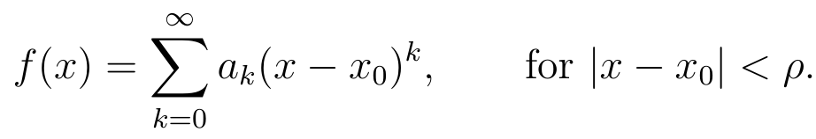
- P , Q , R P,Q,R P,Q,R admit a power series representation around x 0 ∈ R x_0\in R x0∈R
- a function f : I → R (for some interval I) admits a power series representation around x 0 x_0 x0 if
- detailed discussion is coming after this introduction.
- Particularly, we shall see that if P,Q,R admits a power series representation (along with some appropriate conditions), then solutions to the equation (5.1) also admits a power series representation.
- The main issue is of course to determine this power series, particularly, all its coefficients a k ’s.
- Pay attention to our choice of variable.
- We will use the “spatial” variable x as the underlying variable instead of “time” t, as how we used to do that in the previous chapter.
- because a lot of equations of the form (5.1) arise from physical model involving spatial variable, e.g., Airy equation, Bessel equation, e.t.c.


![升级鸿蒙系统效果,鸿蒙系统初体验 全方位体验升级[多图]](https://img-blog.csdnimg.cn/img_convert/802cda68b43696566bcecfef93ae3969.png)