之前做一个小实验写的代码，本想创建个git repo，想了想好像没必要，直接用篇博文记录一下吧。
对应资源： https://download.csdn.net/download/rayso9898/87865298

0. 大纲

0.1 代码说明

dataGeneration.py ->
RSA生成n张图像，可以指定颗粒个数为m,半径为r。
exGraph.py ->
将一张sim仿真图像，转换成一个node_feature matrix, n * 4 : n个节点，3个特征-质心x y,等效直径，面积
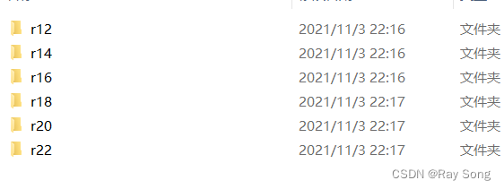
有r12 - r22共 6 种不同粒径的图像，组成字典，每种类别有100张图的node_feature
create_dataset.py ->
主要是 create_graph函数
gcn.py ->
gcn回归模型
task_script ->
提供模型训练预测保存 loss查看等功能

0.2 数据说明

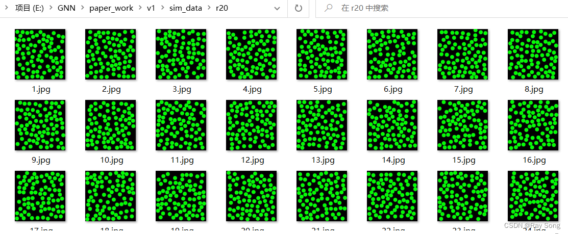
sim_data.zip -> dataGeneration.py 生成
r12-r22共6个文件夹，每个文件夹100张图像。
sim_gdata.pt -> exGraph.py 生成
sim_gdata structure:
all - r12 r14 r16 r18 r20 r22
r12 - img1 img2 … img100
img1 - particle1 … paritle n
particle1 - [x,y,dalimeter,area]
dataset_img_property.pt -> create_dataset.py 生成
x = [] # 图所对应的节点 num4 （x,y,r,area）
pos = []# 图所对应节点的位置 num2 (x,y)
y = stress[i] # 图所对应的力学性能数据
x = torch.tensor(x,dtype=torch.float32)
# 构造一张img的一个图
y = torch.tensor([y],dtype=torch.float32)
pos = torch.tensor(pos,dtype=torch.float32)
edge_index = knn_graph(pos, k=5)
g = Data(x=x, y=y, pos=pos,edge_index=edge_index)
all.append(g)
gcn.pt ->
模型后续加载即可使用
loss_gcn.pt
训练过程中的训练集和测试集loss变化

1. dataGeneration.py ->随机序列吸附法（RSA）生成颗粒图像

可以指定生成颗粒的个数和颗粒半径，以及生成的图像个数。
在这里插入图片描述

# -*- coding: utf-8 -*-
# @Time    : 2021/5/1 15:12
# @Author  : Ray_song
# @File    : dataGeneration.py
# @Software: PyCharmimport cv2
import math
import numpy as npdef calcDis(a,b,c,d):return math.sqrt(math.pow(a-c,2)+math.pow(b-d,2))def generate(n,r,filename,save_path):'''基于RSA算法，生成一张图像:param n: 该图像中有n个颗粒:param r: 颗粒的半径大小为r:param filename: 图像的名字  如 1 2 3 ....:param save_path: 图像的保存路径 - 文件夹:return: None'''# 1.创建白色背景图片d = 512img = np.ones((d, d, 3), np.uint8) * 0#testinglist = []center_x = np.random.randint(0, high=d)center_y = np.random.randint(0, high=d)list.append([center_x,center_y])# 随机半径与颜色radius = rcolor = (0, 255, 0)cv2.circle(img, (center_x, center_y), radius, color, -1)# 2.循环随机绘制实心圆for i in range(1, n):flag = True# 随机中心点while flag:center_x_new = np.random.randint(radius, high=d-radius)center_y_new = np.random.randint(radius, high=d-radius)panduan = Truefor per in list:Dis = calcDis(center_x_new, center_y_new, per[0], per[1])if Dis<2*r:panduan = Falsebreakelse:continueif panduan:list.append([center_x_new,center_y_new])cv2.circle(img, (center_x_new, center_y_new), radius, color, -1)break# 3.显示结果# cv2.imshow("img", img)# cv2.waitKey()# cv2.destroyAllWindows()# 4.保存结果root = f'{save_path}/{filename}.jpg'cv2.imwrite(root,img)def main():# example1 ： 随机生成 100张 颗粒个数为80 半径为20 的 图像save_path = 'sim_data/r20'for i in range(100):generate(80,20,i+1,save_path)if __name__ == '__main__':main()

2. exGraph.py

将一张sim仿真图像，转换成一个node_feature matrix, n * 4 : n个节点，3个特征-质心x y,等效直径，面积
有r12 - r22共 6 种不同粒径的图像，组成字典，每种类别有100张图的node_feature

# -*- coding: utf-8 -*-
# @Time    : 2021/11/3 22:18
# @Author  : Ray_song
# @File    : exGraph.py
# @Software: PyCharmimport os
import torch# 计算面积占比
def countArea(img):# 返回面积占比area = 0size = img.shapeheight,width = size[0],size[1]for i in range(height):for j in range(width):if img[i, j] == 255:area += 1total = height * widthratio = area / totalreturn ratiodef distributionFit(img):'''计算一张照片中所有的 质心坐标xy、颗粒直径、面积，从一张图像中构建graph:param img: RSA生成的图像:return: 图像对应的graph，n*4, n个node, 4个feature'''import numpy as npimport cv2 as cvimg_color = cv.imread(img,1) # countors现实阶段使用img = cv.imread(img,0)# 遍历文件夹中所有的图像thresh_mode = 'THRESH_BINARY+THRESH_OTSU'# 阈值分割内容thresh_down = 127thresh_up = 256if thresh_mode == 'THRESH_BINARY':ret, thresh = cv.threshold(img, thresh_down, thresh_up, cv.THRESH_BINARY)elif thresh_mode == 'THRESH_BINARY_INV':ret, thresh = cv.threshold(img, thresh_down, thresh_up, cv.THRESH_BINARY_INV)elif thresh_mode == 'THRESH_TRUNC':ret, thresh = cv.threshold(img, thresh_down, thresh_up, cv.THRESH_TRUNC)elif thresh_mode == 'THRESH_TOZERO':ret, thresh = cv.threshold(img, thresh_down, thresh_up, cv.THRESH_TOZERO)elif thresh_mode == 'THRESH_TOZERO_INV':ret, thresh = cv.threshold(img, thresh_down, thresh_up, cv.THRESH_TOZERO_INV)elif thresh_mode == 'THRESH_BINARY+THRESH_OTSU':ret, thresh = cv.threshold(img, thresh_down, thresh_up, cv.THRESH_BINARY + cv.THRESH_OTSU)elif thresh_mode == 'No':thresh = imgcontours, hierarchy = cv.findContours(thresh, cv.RETR_EXTERNAL, cv.CHAIN_APPROX_NONE)# 显示contours的代码，可以取消注释进行显示# cv.drawContours(img_color,contours,-1,(255,0,0),1)# cv.imshow('1',img_color)# cv.waitKey(0)graph = []for i in range(len(contours)):node = []cnt = contours[i]M = cv.moments(cnt)  # 计算图像矩# print(M)cx = int(M['m10'] / M['m00'])  # 重心的x坐标cy = int(M['m01'] / M['m00'])  # 重心的y坐标area = cv.contourArea(cnt)equi_diameter = np.sqrt(4 * area / np.pi)node.append(cx)node.append(cy)node.append(equi_diameter)node.append(area)graph.append(node)return graphdef exGraph():dirs = os.listdir('./sim_data')print(dirs)sim_data = {}list = ['r12','r14','r16','r18','r20','r22']index = 0for dir in dirs:path = r'sim_data'+'//'+dir# path = './sim_data/r12'imgs = os.listdir(path)print(len(imgs))con = []for i in range(len(imgs)):img_path = path+'/'+imgs[i]graph = distributionFit(img_path)con.append(graph)sim_data[list[index]] = conindex = index+1torch.save(sim_data,'sim_gdata.pt')if __name__ == '__main__':a = torch.load('./sim_gdata.pt')print(a)

3. create_dataset.py ->

主要是 create_graph函数

# -*- coding: utf-8 -*-
# @Time    : 2021/11/4 23:01
# @Author  : Ray_song
# @File    : create_dataset.py
# @Software: PyCharmimport torch
from torch_geometric.data import Data
from torch_cluster import knn_graph'''sim_gdata structure:all - r12  r14  r16  r18 r20 r22r12 - img1 img2 ... img100img1 - particle1 .. paritle nparticle1 - [x,y,dalimeter,area]
'''def create_graph():path = r'./sim_gdata.pt'data = torch.load(path)r = ['r12', 'r14', 'r16', 'r18', 'r20', 'r22']stress = [225, 230, 235, 240, 245, 250, 255]# 构造图all = []for i in range(len(data)):ri = r[i] # 字典 - 图数据的字典imgs = data[ri]y = stress[i]  # 图所对应的力学性能数据# 遍历ri中的每一张图for j in range(len(imgs)):x = [] # 图所对应的节点 num*4 （x,y,r,area）pos = []# 图所对应节点的位置 num*2  (x,y)img = imgs[j]# 遍历图中所有的节点for k in range(len(img)):# 单个节点的特征xi = []xi.append(img[k][0])xi.append(img[k][1])xi.append(img[k][2])xi.append(img[k][3])x.append(xi)# 位置信息(x,y)posi = []posi.append(img[k][0])posi.append(img[k][1])pos.append(posi)x = torch.tensor(x,dtype=torch.float32)# 构造一张img的一个图y = torch.tensor([y],dtype=torch.float32)pos = torch.tensor(pos,dtype=torch.float32)g = Data(x=x, y=y, pos=pos)g.edge_index = knn_graph(pos, k=5)all.append(g)torch.save(all,r'dataset_img_property.pt')return allif __name__ == '__main__':create_graph()

4. gcn.py ->

gcn回归模型


# -*- coding: utf-8 -*-
# @Time    : 2021/11/5 19:13
# @Author  : Ray_song
# @File    : gcn.py
# @Software: PyCharmimport torch
from torch.nn import Linear
from torch_geometric.nn import GCNConv
from torch_geometric.nn import global_mean_poolclass GCN(torch.nn.Module):def __init__(self, hidden_channels):super(GCN, self).__init__()# torch.manual_seed(12345)self.conv1 = GCNConv(4, hidden_channels)self.conv2 = GCNConv(hidden_channels, hidden_channels)# self.conv3 = GCNConv(hidden_channels, hidden_channels)self.lin = Linear(hidden_channels, 1)def forward(self, x, edge_index, batch):# 1. Obtain node embeddingsx = self.conv1(x, edge_index)x = x.relu()x = self.conv2(x, edge_index)# x = x.relu()# x = self.conv3(x, edge_index)# 2. Readout layerx = global_mean_pool(x, batch)  # [batch_size, hidden_channels]# 3. Apply a final regressorx = self.lin(x)return x

5. task_script ->

提供模型训练 预测保存 loss查看等功能

import numpy as np
import pandas as pd
import torch
# from torch_geometric.data import Data
# from torch_cluster import knn_graph
# import matplotlib.pyplot as plt
# from mpl_toolkits.mplot3d import Axes3D
# from torch_geometric.datasets import GeometricShapes
# from torch_cluster import knn_graph
from torch_geometric.loader import DataLoader
from gcn import GCN,GCNConvdef showDataset():path = r'./dataset_img_property.pt'dataset = torch.load(path)print()# print(f'Dataset: {dataset}:')print('====================')print(f'Number of graphs: {len(dataset)}')# print(f'Number of features: {dataset.num_features}')# print(f'Number of classes: {dataset.num_classes}')data = dataset[0]  # Get the first graph object.print()print(data)print('=============================================================')# Gather some statistics about the first graph.print(f'Number of nodes: {data.num_nodes}')print(f'Number of edges: {data.num_edges}')print(f'Average node degree: {data.num_edges / data.num_nodes:.2f}')print(f'Has isolated nodes: {data.has_isolated_nodes()}')print(f'Has self-loops: {data.has_self_loops()}')# print(f'Is undirected: {data.is_undirected()}')def split_train_val(path):dataset = torch.load(path)import randomrandom.shuffle(dataset)num = len(dataset)# print(dataset,num)ratio = 0.8train_dataset = dataset[:int(num*ratio)]val_dataset = dataset[int(num*ratio):]print(len(train_dataset),len(val_dataset))return train_dataset,val_datasetdef begin():import torchpath = r'./dataset_img_property.pt'dataset = torch.load(path)train_dataset,test_dataset = split_train_val(path)train_loader = DataLoader(train_dataset, batch_size=32, shuffle=True)test_loader = DataLoader(test_dataset, batch_size=32, shuffle=False)model = GCN(hidden_channels=64)print(model)optimizer = torch.optim.Adam(model.parameters(), lr=0.001,weight_decay=1e-8)criterion = torch.nn.MSELoss()def train():model.train()train_loss = 0for data in train_loader:  # Iterate in batches over the training dataset.out = model(data.x, data.edge_index, data.batch)  # Perform a single forward pass.loss = criterion(out.squeeze(-1), data.y)  # Compute the loss.train_loss = train_loss + loss.item()# print(f'train_loss:{train_loss/data.batch}')loss.backward()  # Derive gradients.optimizer.step()  # Update parameters based on gradients.optimizer.zero_grad()  # Clear gradients.def test(loader):model.eval()loss_ = 0count = 0for data in loader:  # Iterate in batches over the training/test dataset.out = model(data.x, data.edge_index, data.batch)loss = criterion(out.squeeze(-1), data.y)loss_ += loss.item()count += 1return loss_/countloss_t = []loss_v = []for epoch in range(1, 300):loss = []train()train_acc = test(train_loader)test_acc = test(test_loader)if test_acc<45:torch.save(model.state_dict(),'./gcn.pt')loss_t.append(train_acc)loss_v.append(test_acc)print(f'Epoch: {epoch:03d}, Train Acc: {train_acc:.4f}, Test Acc: {test_acc:.4f}')loss.append(loss_t)loss.append(loss_v)torch.save(loss,'loss_gcn.pt')def draw_loss():import matplotlib.pyplot as pltloss = torch.load('loss_gcn.pt')plt.plot(loss[0])plt.plot(loss[1])plt.show()def prediction_all():from sklearn.metrics import mean_squared_errorprediction_classes = 1g_path = r'./dataset_img_property.pt'save_path = r'./prediction.csv'g_data = torch.load(g_path)model = GCN(hidden_channels=64)model_weight = r'./gcn.pt'model.load_state_dict(torch.load(model_weight))model.eval()# begin predicting...res = []val_data = g_data[:600]pre_dataloader = DataLoader(val_data, batch_size=1)y = []with torch.no_grad():for item in pre_dataloader:# predict classy.append(item.y.item())output = torch.squeeze(model(item.x,item.edge_index,item.batch))  # 将batch维度压缩掉prediction = output.numpy()if prediction_classes > 1:prediction = list(prediction)res.append(prediction)res = np.array(res)y = np.array(y)acc = mean_squared_error(res,y)print('acc',acc)res = pd.DataFrame(res)res.to_csv(save_path,header=None,index=None)if __name__ == '__main__':prediction_all()