Week 02 of Advanced Learning Algorithms
笔者在2022年7月份取得这门课的证书,现在(2024年2月25日)才想起来将笔记发布到博客上。
Website: https://www.coursera.org/learn/advanced-learning-algorithms?specialization=machine-learning-introduction
Offered by: DeepLearning.AI and Stanford

课程地址:https://www.coursera.org/learn/machine-learning
本笔记包含字幕,quiz的答案以及作业的代码,仅供个人学习使用,如有侵权,请联系删除。
文章目录
- Week 02 of Advanced Learning Algorithms
- Learning Objectives
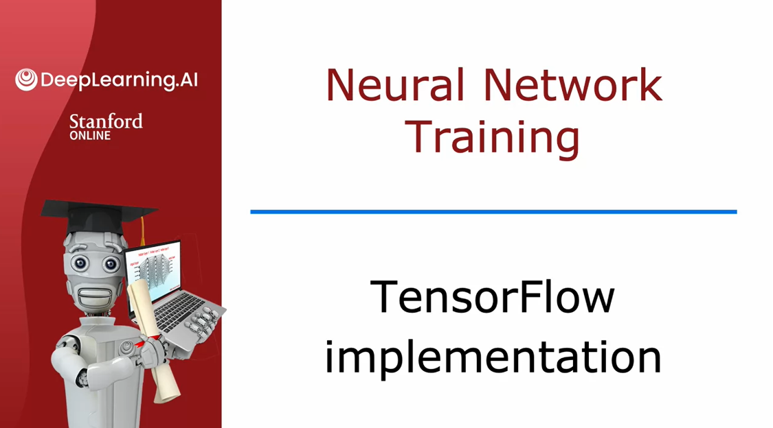
- [1] Neural Network Training
- TensorFlow implementation
- Training Details
- [2] Practice quiz: Neural Network Training
- [3] Activation Functions
- Alternatives to the sigmoid activation
- Choosing activation functions
- Compare ReLU with Sigmoid
- Why do we need activation functions?
- Lab: ReLU activation
- Why Non-Linear Activations?
- [4] Practice quiz: Activation Functions
- [5] Multiclass Classification
- Multiclass
- Softmax
- Neural Network with Softmax output
- Improved implementation of softmax
- Classification with multiple outputs (Optional)
- Lab: Softmax
- Softmax Function
- Cost
- Tensorflow
- The *Obvious* organization
- Preferred
- Output Handling
- SparseCategorialCrossentropy or CategoricalCrossEntropy
- Congratulations!
- Lab: Multiclass
- 1.1 Goals
- 1.2 Tools
- 2.0 Multi-class Classification
- 2.1 Prepare and visualize our data
- 2.2 Model
- Explanation
- Layer 1
- Layer 2, the output layer
- [6] Practice quiz: Multiclass Classification
- [7] Additional Neural Network Concepts
- Advanced Optimization
- Additional Layer Types
- [8] Practice quiz: Additional Neural Network Concepts
- [9] Practice Lab: Neural network training
- 1 - Packages
- 2 - ReLU Activation
- 3 - Softmax Function
- Exercise 1
- 4 - Neural Networks
- 4.1 Problem Statement
- 4.2 Dataset
- 4.2.1 View the variables
- 4.2.2 Check the dimensions of your variables
- 4.2.3 Visualizing the Data
- 4.3 Model representation
- 4.4 Tensorflow Model Implementation
- 4.5 Softmax placement
- Exercise 2
- Epochs and batches
- Loss (cost)
- Prediction
- Congratulations!
- 其他
- 英文发音
This week, you’ll learn how to train your model in TensorFlow, and also learn about other important activation functions (besides the sigmoid function), and where to use each type in a neural network.
You’ll also learn how to go beyond binary classification to multiclass classification (3 or more categories).
Multiclass classification will introduce you to a new activation function and a new loss function.
Optionally, you can also learn about the difference between multiclass classification and multi-label classification.
You’ll learn about the Adam optimizer, and why it’s an improvement upon regular gradient descent for neural network training.
Finally, get a brief introduction to other layer types besides the one you’ve seen thus far.
Learning Objectives
- Train a neural network on data using TensorFlow
- Understand the difference between various activation functions (sigmoid, ReLU, and linear)
- Understand which activation functions to use for which type of layer
- Understand why we need non-linear activation functions
- Understand multiclass classification
- Calculate the softmax activation for implementing multiclass classification
- Use the categorical cross entropy loss function for multiclass classification
- Use the recommended method for implementing multiclass classification in code
- (Optional): Explain the difference between multi-label and multiclass classification
[1] Neural Network Training
TensorFlow implementation
Welcome back to
the second week of this course on advanced
learning algorithms.Last week, you learned how to carry out inference
on a neural network.This week, we’re going to go over training of
a neural network.I think being able to
take you on data and train you on neural network
unit is really fun. This week, we’ll look at how you could do that. Let’s dive in.
Let’s continue with
our running example of hand written
digit recognition, recognizing this image
as zero or a one.
Here we are using the neural network architecture
that you saw last week where you
have an input X, that is the image, and then the first sitting
there with 25 units, second sitting there
with 15 units, and then one operate unit.
How to train the parameters of a neural network?
If you are given a
training set of examples comprising images X as was
the ground proof labeled Y, how would you train the
parameters of this new network?
Just take a look at the code
Dive in the details in the next few videos
Let me go ahead and show
you the code that you can use in TensorFlow
to train this network, and then in the next
few videos after this, we’ll dive in the details explaining what the
code is actually doing.This is the code you write.
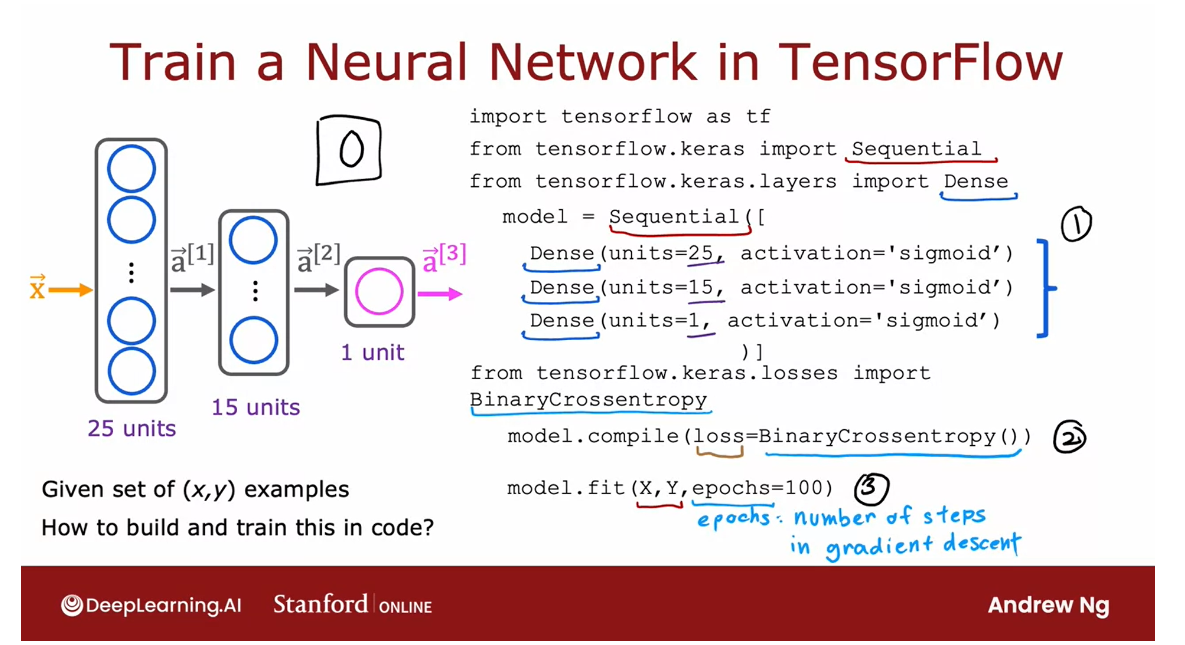
The first step: Build a model, string different layers sequentially
This first part may look familiar from the previous week, where you are asking
TensorFlow to sequentially string together these three
layers of a neural network.The first in the layer with 25 units and sigmoid activation, the second [inaudible] there, and then finally,
the upper layer.Nothing new here relative
to what you saw last week.
The second step: Compile the model
Second step is you have
to ask TensorFlow to compile the model and the key step in asking TensorFlow to compile
the mode is to specify what is the last
function you want to use.
Arcane name: sparse categorical cross entropy
In this case, we’ll use
something that goes by the arcane name of sparse
categorical cross entropy.We’ll see more in the
next video what this is.
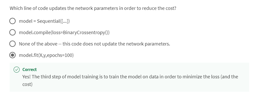
The third step: Call the fit function to fit the model
Then having specified
the last function, the next step is to call the fit function which tells
TensorFlow to fit the model that you specified in
step 1 using the last of the cost function that
you specified in step 2 to the data set XY.
Back in the first
course is when we talked about creating descent.We had to decide how many
steps to run creating descent, so how long to run
creating descent.
Epoch is a technical
term for how many steps creating descent that you
may want to run. That’s it.
Step 1 is to specify
the mode which tells TensorFlow how to compute
for the inference.Step 2… (TIME COULD NOT ALLOW ME TO FINISH). Our p whenever things don’t work the way you expect.
With that, let’s go on to the next video where
we’ll dive more deeply into what these steps in the TensorFlow implementation
are actually doing. I’ll see you in the next video.
Training Details
Let’s take a look at the details of what the TensorFlow code for training a neural network is actually doing. Let’s dive in.
Before looking at the details of training in neural network, let’s recall how you had trained a logistic regression model
in the previous course.
How to build a logistic regression model?
Step 1: specify how to compute output given input and parameters W and B
Step 1 of building a logistic regression
model was you would specify how to
compute the output given the input feature x
and the parameters w and b.In the first course we said the logistic regression function predicts f of x is equal to G. The sigmoid function applied
to W. product X plus B which was the sigmoid function
applied to W.X plus B.
If Z is the dot product
of W of X plus B, then F of X is 1 over 1
plus e to the negative z, so those first step were to
specify what is the input to output function of
logistic regression, and that depends on
both the input x and the parameters of the model.
Step 2: specify loss and cost
The second step we
had to do to train the literacy regression
model was to specify the loss function
and also the cost function, so you may recall that
the loss function said, if religious regression opus f of x and the ground truth label, the actual label and
a training set was y then the loss on that
single training example was negative y log f of x minus one minus y times log
of one minus f of x.
Loss function: a measure of how well is logistic regression doing on a single training example
This was a measure of how
well is logistic regression doing on a single training
example x comma y.
Cost function: an average of the loss function computed over the entire training set
Given this definition
of a loss function, we then define the
cost function, and the cost function
was a function of the parameters W and B, and that was just the
average that is taking an average overall M
training examples of the loss function computed on the M training examples,
X1, Y1 through XM YM, and remember that in
the convention we’re using the loss function is
a function of the output of the learning algorithm and
the ground truth label as computed over a single
training example whereas the cost function J is an average of the loss function computed over your
entire training set.That was step two of what we did when building up
logistic regression.
Step 3: train on data to minimize the cost function J
Then the third and
final step to train a logistic regression model
was to use an algorithm specifically gradient descent to minimize that cost function J of WB to minimize it as a function of the
parameters W and B.
We minimize the cost
J as a function of the parameters using
gradient descent where W is updated as W minus
the learning rate alpha times the derivative
of J with respect to W.
And B similarly is updated as B minus the learning rate alpha times the derivative of
J with respect to B.
If these three steps.
Step one, specifying
how to compute the outputs given the
input X and parameters, step 2 specify loss and costs, and step three minimize the cost function we trained
logistic regression.
The same three
steps is how we can train a neural network
in TensorFlow.Now let’s look at how
these three steps map to training a
neural network.We’ll go over this
in greater detail on the next three slides
but really briefly.
Step one is specify how to compute the output
given the input x and parameters W and B
that’s done with this code snippet which
should be familiar from last week of specifying the neural network and this
was actually enough to specify the
computations needed in forward propagation or for the inference
algorithm for example.
The second step is to compile the model and to tell it
what loss you want to use, and here’s the code
that you use to specify this loss function which is the binary cross
entropy loss function, and once you specify this
loss taking an average over the entire training
set also gives you the cost function
for the neural network, and then step three is to
call function to try to minimize the cost as a function of the parameters
of the neural network.
Let’s look in greater detail in these three steps in the context of training
a neural network.
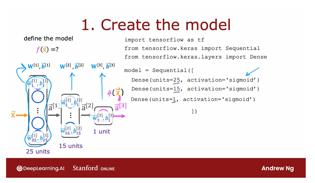
1 Create the model
The first step,
specify how to compute the output given the input
x and parameters w and b.
This code snippet specifies the entire architecture
of the neural network.It tells you that there are 25 hidden units in the
first hidden layer, then the 15 in the next one, and then one output unit and that we’re using the
sigmoid activation value.
Based on this code snippet, we know also what are
the parameters w1, v1 though the first
layer parameters of the second layer and
parameters of the third layer.
This code snippet specifies the entire architecture of the neural network and therefore tells TensorFlow
everything it needs in order to compute the
output x as a function.
In order to compute
the output a 3 or f of x as a function of the
input x and the parameters, here we have written w l and
b l.
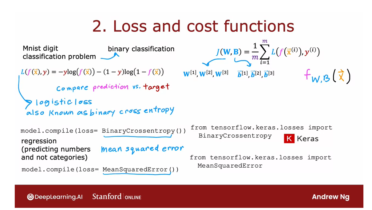
2 Loss and cost function
Let’s go on to step 2. In the second step, you have to specify what
is the loss function.That will also define the cost function we use to
train the neural network.
For the m is 01 digit classification
problem is a binary classification problem
and most common by far, our loss function to use
is this one is actually the same loss function
as what we had for logistic regression is
negative y log f of x minus 1 minus y times
log 1 minus f of x, where y is the
ground truth label, sometimes also called
the target label y, and f of x is now the output
of the neural network.
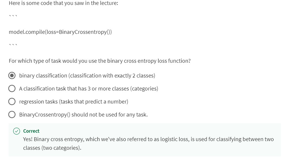
Binary cross entropy loss function
In the terminology
of TensorFlow, this loss function is called
binary cross entropy.The syntax is to
ask TensorFlow to compile the neural network
using this loss function.
Another historical note, keras was originally
a library that had developed independently of TensorFlow is actually totally separate project
from TensorFlow.But eventually it got
merged into TensorFlow, which is why we have tf.Keras library.losses dot the name
of this loss function.
By the way, I don’t
always remember the names of all the loss
functions and TensorFlow, but I just do a quick
web search myself to find the right name and then
I plug that into my code.
Having specified the loss with respect to a single
training example, TensorFlow knows that
it costs you want to minimize is then the average, taking the average over all m training examples of the loss on all of the
training examples.
Optimizing this cost
function will result in fitting the neural network to your binary classification data.In case you want to solve a regression problem rather than a classification problem.
You can also tell
TensorFlow to compile your model using a
different loss function.
Regression problem loss function: squared error loss
For example, if you have a regression problem and if you want to minimize
the squared error loss.Here is the squared error loss.
The loss with respect to if your learning
algorithm outputs f of x with a target or
ground truth label of y, that’s 1.5 of the squared error.Then you can use this loss
function in TensorFlow, which is to use the maybe more
intuitively named mean squared error loss function.Then TensorFlow will try to minimize the mean squared error.
In this expression, I’m
using j of capital w comma capital b to denote
the cost function.The cost function is a function of all the parameters
into neural network. You can think of capital W
as including W1, W2, W3.
All the W parameters and the
entire new network and be as including b1, b2, and b3. If you are optimizing the cost function
respect to w and b, if we tried to optimize
it with respect to all of the parameters
in the neural network.
Up on top as well, I had written f of x as the
output of the neural network, but we can also write f of w p if we want to emphasize that the output of the neural network as a function of x depends on all the parameters in all the layers of
the neural network.
That’s the loss function
and the cost function.In TensorFlow,
this is called the binary cross-entropy
loss function.
Where does that name come from?
Well, it turns out in
statistics this function on top is called the
cross-entropy loss function, so that’s what
cross-entropy means, and the word binary just reemphasizes or
points out that this is a binary classification
problem because each image is either
a zero or a one.
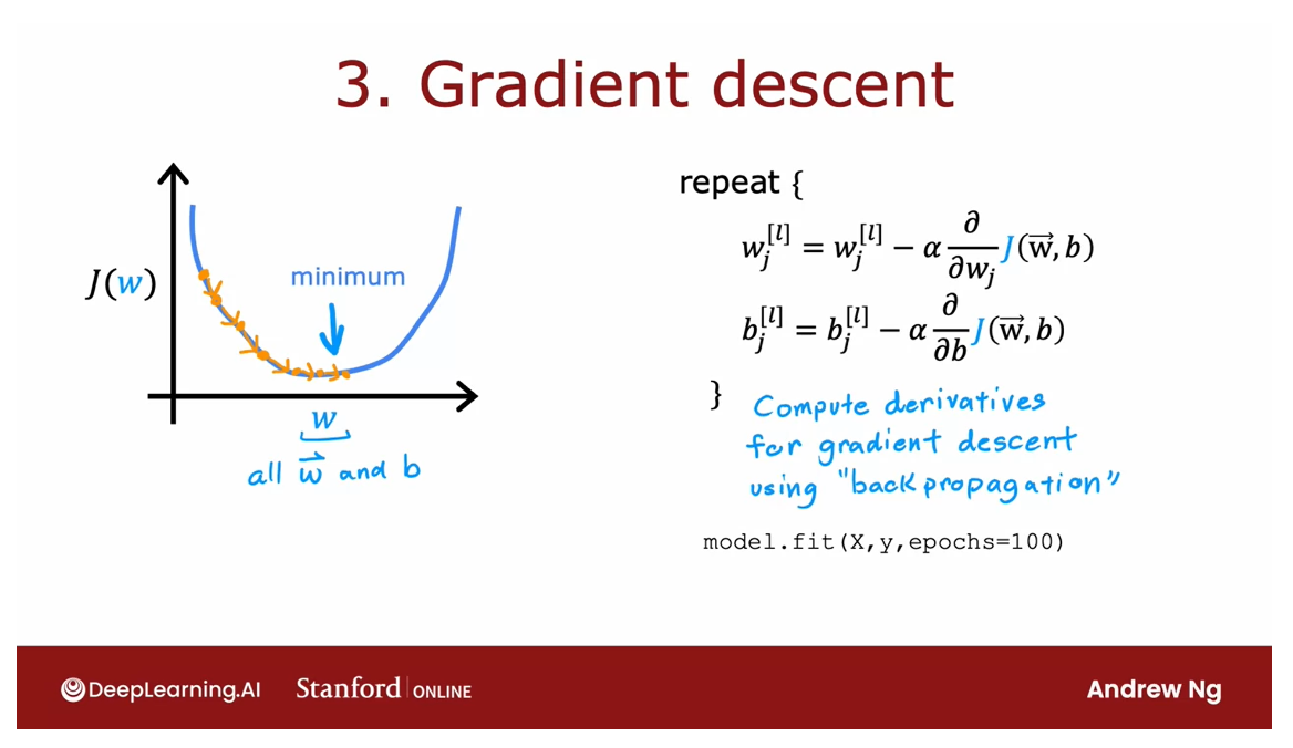
3 Gradient descent
Minimize the cost function
Finally, you will ask TensorFlow to minimize
the cost function. You might remember the
gradient descent algorithm from the first course.
If you’re using
gradient descent to train the parameters
of a neural network, then you are repeatedly, for every layer l and
for every unit j, update wlj according to wlj minus the learning rate alpha times the
partial derivative with respect to that parameter
of the cost function j of wb and similarly for
the parameters b as well.
After doing, say, 100 iterations of gradient
descent, hopefully, you get to a good value
of the parameters.
In order to use
gradient descent, the key thing you need to compute is these partial
derivative terms.
Compute partial derivatives: use back propagation
What TensorFlow does, and, in fact, what is standard
in neural network training, is to use an algorithm
called back propagation in order to compute these
partial derivative terms.
TensorFlow can do all of
these things for you. It implements
backpropagation all within this function called fit.
All you have to do is
call model.fit, x, y as your training set, and tell it to do so for 100
iterations or 100 epochs.
In fact, what you see later
is that TensorFlow can use an algorithm that
is even a little bit faster than
gradient descent, and you’ll see more about
that later this week as well.
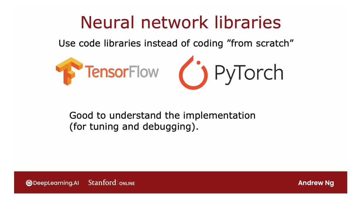
Now, I know that we’re
relying heavily on the TensorFlow library in order to implement a neural network.
libraries become more mature
One pattern I’ve seen across multiple ideas is as
the technology evolves, libraries become more mature, and most engineers
will use libraries rather than implement
code from scratch.
There have been
many other examples of this in the
history of computing.
Once, many decades ago, programmers had to implement their own sorting
function from scratch, but now sorting
libraries are quite mature that you probably call someone else’s
sorting function rather than implement
it yourself, unless you’re taking a
computing class and I ask you to do it as an exercise.
Today, if you want to compute the square
root of a number, like what is the square
root of seven, well, once programmers had to write their own code
to compute this, but now pretty
much everyone just calls a library to
take square roots, or matrix operations, such as multiplying
two matrices together.
When deep learning was young: implement things from scratch
When deep learning was
younger and less mature, many developers, including me, were implementing
things from scratch using Python or C++ or
some other library.
Today, deep learning libraries have matured enough
But today, deep learning
libraries have matured enough that most developers
will use these libraries, and, in fact, most commercial implementations
of neural networks today use a library like
TensorFlow or PyTorch.
It’s still useful to understand how they work under the hood
But as I’ve mentioned, it’s still useful to
understand how they work under the hood so that if something
unexpected happens, which still does with
today’s libraries, you have a better chance
of knowing how to fix it.
Now that you know how to
train a basic neural network, also called a
multilayer perceptron, there are some things
you can change about the neural network that will
make it even more powerful.
In the next video, let’s take a look
at how you can swap in different
activation functions as an alternative to the sigmoid activation
function we’ve been using. This will make your
neural networks work even much better. Let’s go take a look at
that in the next video.
[2] Practice quiz: Neural Network Training
Practice quiz: Neural Network Training
Latest Submission Grade 100%
Question 1
Binary cross entropy, which we’ve also referred to as logistic loss, is used for classifying between two classes (two categories).
Question 2
[3] Activation Functions
Alternatives to the sigmoid activation
Demand prediction: use sigmoid activation function
So far, we’ve been using the sigmoid
activation function in all the nodes in the hidden layers and in the output layer.And we have started that way
because we were building up neural networks by taking
logistic regression and creating a lot of logistic regression
units and string them together.
But if you use other activation functions, your neural network can
become much more powerful.Let’s take a look at how to do that.
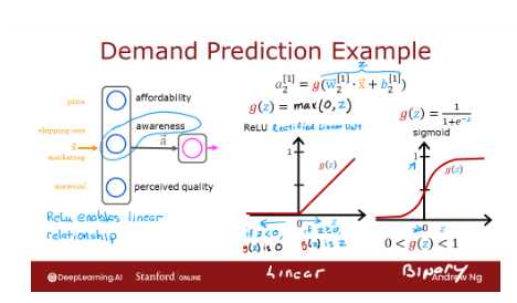
Recall the demand prediction example
from last week where given price, shipping cost, marketing, material, you would try to predict if
something is highly affordable.
If there’s good awareness and
high perceived quality and based on that try to predict
it was a top seller. But this assumes that awareness is maybe
binary is either people are aware or they are not.
But it seems like the degree to which
possible buyers are aware of the t shirt you’re selling may not be binary,
they can be a little bit aware, somewhat aware, extremely aware or
it could have gone completely viral.
So rather than modeling
awareness as a tiny number 0, 1, that you try to estimate
the probability of awareness or rather than modeling awareness is
just a number between 0 and 1.Maybe awareness should be any non negative
number because there can be any non negative value of awareness going
from 0 up to very very large numbers.
So whereas previously we had
used this equation to calculate the activation of that second
hidden unit estimating awareness where g was the sigmoid function and
just goes between 0 and 1.
If you want to allow a,1, 2 to potentially
take on much larger positive values, we can instead swap in
a different activation function.
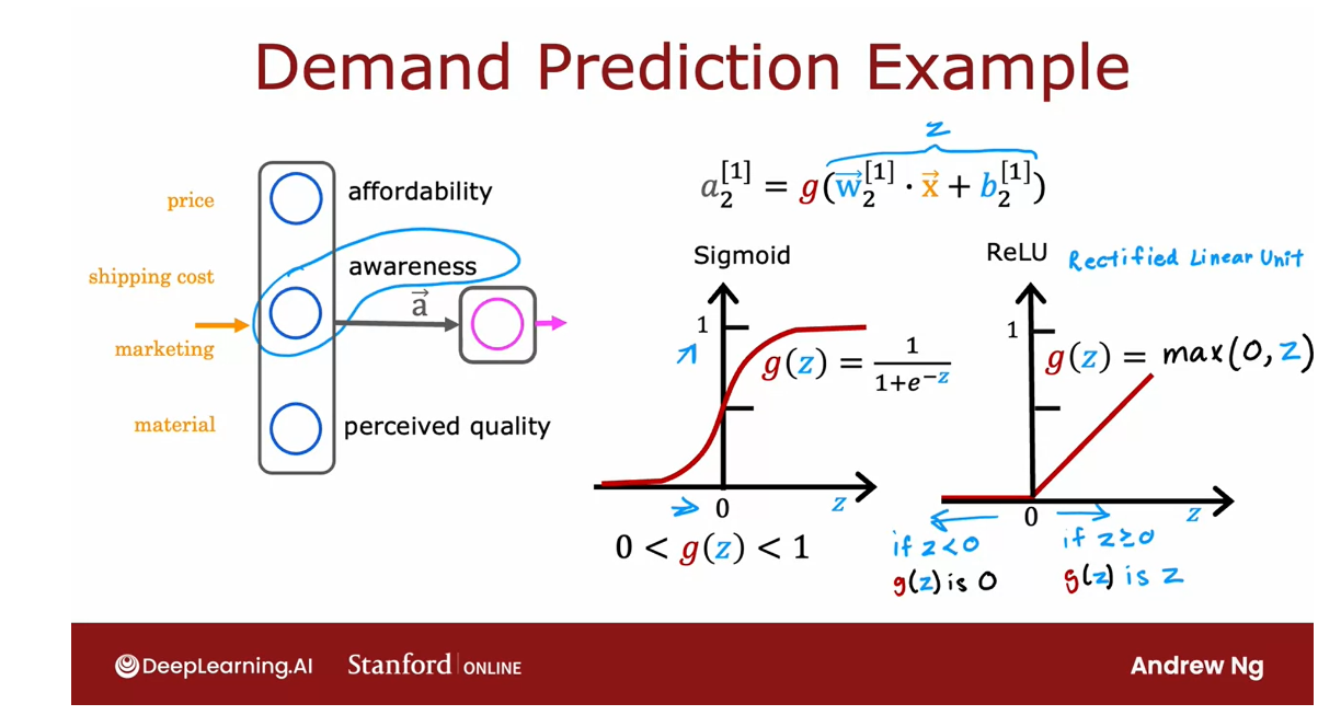
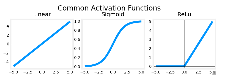
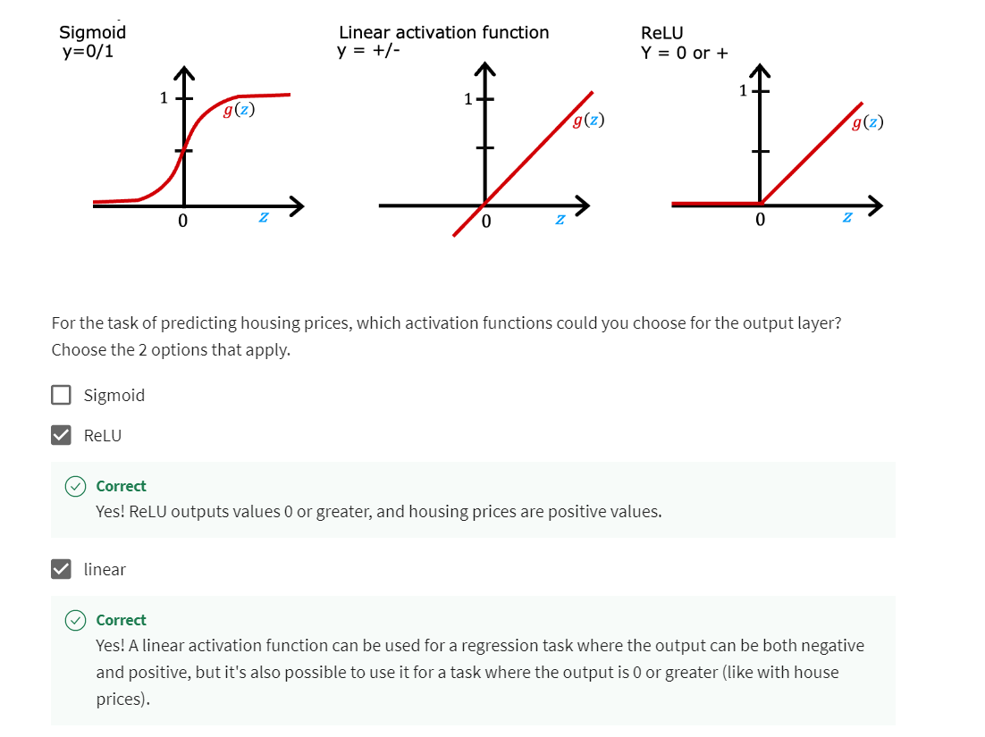
Examples of Activation Functions
ReLU activation function diagram
It turns out that a very common
choice of activation function in neural networks is this function. It looks like this. It goes if z is this,
then g(z) is 0 to the left and then there’s this straight
line 45° to the right of 0.And so when z is greater than or
equal to 0, g(z) is just equal to z. That is to the right half of this diagram.
And the mathematical equation for
this is g(z) equals max(0, z).Feel free to verify for
yourself that max(0, z) results in this curve
that I’ve drawn over here. And if a 1, 2 is g(z) for
this value of z, then a, the deactivation value cannot take on 0 or
any non negative value.
ReLU activation function
This activation function has a name. It goes by the name ReLU with this funny
capitalization and ReLU stands for again, somewhat arcane term, but
it stands for rectified linear unit.
Don’t worry too much about what rectified
means and what linear unit means. This was just the name that
the authors had given to this particular activation function
when they came up with it.
But most people in deep learning
just say ReLU to refer to this g(z). More generally you have a choice
of what to use for g(z) and sometimes we’ll use a different choice
than the sigmoid activation function.
Here are the most commonly
used activation functions. You saw the sigmoid activation function,
g(z) equals this sigmoid function.On the last slide we just
looked at the ReLU or rectified linear unit g(z) equals max(0,
z).
One other activation function which is worth mentioning: linear activation function
There’s one other activation
function which is worth mentioning, which is called the linear activation
function, which is just g(z) equals to z.
Sometimes if you use the linear
activation function, people will say we’re not using
any activation function because if a is g(z) where g(z) equals z,
then a is just equal to this w.x plus b z.
And so
it’s as if there was no g in there at all. So when you are using this linear
activation function g(z) sometimes people say, well,
we’re not using any activation function.
Although in this class, I will refer
to using the linear activation function rather than no activation function.
But if you hear someone else use that
terminology, that’s what they mean. It just refers to the linear
activation function.
Later: softmax activation function
And these three are probably
by far the most commonly used activation functions in neural networks.Later this week, we’ll touch on the fourth one called
the softmax activation function.
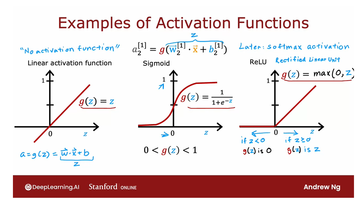
But with these activation
functions you’ll be able to build a rich variety of
powerful neural networks.
How to choose activation function?
So when building a neural network for
each neuron, do you want to use the signal activation
function or the ReLU activation function? Or a linear activation function? How do you choose between these
different activation functions? Let’s take a look at
that in the next video.
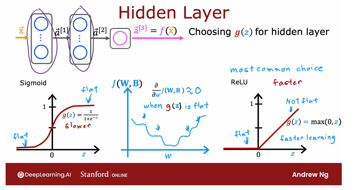
Choosing activation functions
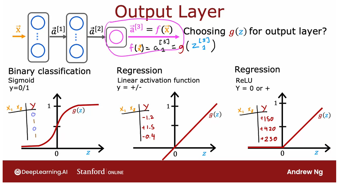
Output Layer
Let’s take a look at
how you can choose the activation function for different neurons in
your neural network.
Choose activation function for output layer
We’ll start with some
guidance for how to choose it for
the output layer.
It turns out that
depending on what the target label or the
ground truth label y is, there will be one
fairly natural choice for the activation function
for the output layer, and we’ll then go and
look at the choice of the activation function also for the hidden layers of
your neural network. Let’s take a look.
You can choose different activation
functions for different neurons in
your neural network, and when considering
the activation function for the output layer, it turns out that there’ll often be one fairly natural choice, depending on what is the target or the
ground truth label y.
Specifically, if
you are working on a classification problem where
y is either zero or one, so a binary
classification problem, then the sigmoid
activation function will almost always be
the most natural choice, because then the neural
network learns to predict the probability
that y is equal to one, just like we had for
logistic regression.
Binary classification problem, use sigmoid at the output layer
My recommendation is, if you’re working on a binary
classification problem, use sigmoid at the output layer.
Regression problem
Alternatively, if you’re
solving a regression problem, then you might choose a
different activation function.
Predict how tomorrow’s stock price
A number that can be either positive or negative: linear activation function
For example, if you are
trying to predict how tomorrow’s stock price will change compared to
today’s stock price.Well, it can go up or down, and so in this case y
would be a number that can be either positive or negative, and in that case
I would recommend you use the linear
activation function.
Why is that? Well, that’s because then the outputs
of your neural network, f of x, which is equal to
a^3 in the example above, would be g applied to z^3 and with the linear
activation function, g of z can take on either
positive or negative values.So y can be positive
or negative, use a linear
activation function.
Predict the price of a house: never be negative
ReLU
Finally, if y can only take
on non-negative values, such as if you’re predicting
the price of a house, that can never be negative, then the most natural
choice will be the ReLU activation function
because as you see here, this activation function only takes on non-negative values, either zero or positive values.
Depending on what is the label y you are trying to predict.
In choosing the
activation function to use for your output layer, usually depending on what is the label y you’re
trying to predict, there’ll be one fairly
natural choice.
In fact, the guidance on
this slide is how I pretty much always choose my
activation function as well for the output
layer of a neural network.
Hidden Layer
Most common choice: ReLU
Choose activation function for hidden layer
How about the hidden layers
of a neural network?
the ReLU activation function is by far the most common choice
It turns out that the ReLU
activation function is by far the most common choice
in how neural networks are trained by many
practitioners today.
Even though we had initially
described neural networks using the sigmoid activation
function, and in fact, in the early history of the development of
neural networks, people use sigmoid activation
functions in many places, the field has evolved to use ReLU much more often and
sigmoids hardly ever.
Well, the one exception
that you do use a sigmoid activation function in the output layer if you have a binary classification problem.
So why is that? Well,
there are a few reasons.
Compare ReLU with Sigmoid
- ReLU is a bit faster to compute
- ReLU function goes flat only in one part of the graph; Sigmoid function goes flat in two places, and the gradient descent would be very slow.
First, if you compare the ReLU and the sigmoid
activation functions, the ReLU is a bit faster
to compute because it just requires
computing max of 0, z, whereas the sigmoid
requires taking an exponentiation and
then a inverse and so on, and so it’s a little
bit less efficient.
But the second
reason which turns out to be even more
important is that the ReLU function goes flat only in one
part of the graph;here on the left is
completely flat, whereas the sigmoid
activation function, it goes flat in two places.
It goes flat to the
left of the graph and it goes flat to the
right of the graph. If you’re using gradient descent to train a neural network, then when you have a function that is fat
in a lot of places, gradient descents
would be really slow.
尽管梯度下降优化的是cost function,而不是优化激活函数。
但是激活函数是需要计算的一部分,这就导致了cost function 中的很多地方是平的,导致梯度下降很慢。
I know that gradient descent optimizes the cost
function J of W, B rather than optimizes
the activation function, but the activation function is a piece of what goes
into computing, and that results in more places in the cost function J of W, B that are flats
as well and with a small gradient and it
slows down learning.
I know that that was just
an intuitive explanation, but researchers have
found that using the ReLU activation
function can cause your neural network to
learn a bit faster as well, which is why for most
practitioners if you’re trying to decide what activation functions to use with hidden layer, the ReLU activation function has become now by far the
most common choice.
In fact that I’m building
a neural network, this is how I choose activation functions for
the hidden layers as well.
Choosing Activation Summary
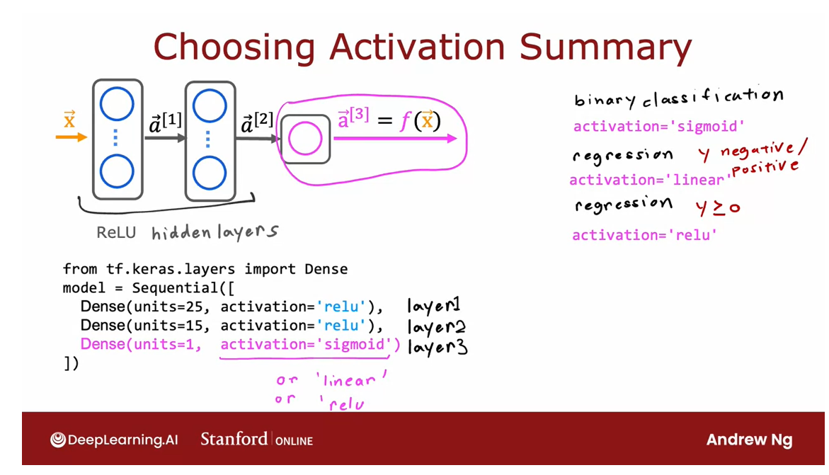
To summarize, here’s what
I recommend in terms of how you choose the activation functions
for your neural network.
For the output layer, use a sigmoid, if you have a binary
classification problem; linear, if y is a number that can take on positive
or negative values, or use ReLU if y can take on only positive values or zero positive values or
non-negative values.
Then for the hidden
layers I would recommend just using ReLU as a default
activation function, and in TensorFlow, this is
how you would implement it.
Rather than saying
activation equals sigmoid as we had previously, for the hidden layers, that’s the first hidden layer, the second hidden layer as TensorFlow to use the
ReLU activation function, and then for the output
layer in this example, I’ve asked it to use the
sigmoid activation function, but if you wanted to use the
linear activation function, is that, that’s
the syntax for it, or if you wanted to use the ReLU activation function that shows the syntax for it.
With this richer set of
activation functions, you’ll be
well-positioned to build much more powerful
neural networks than just once using only the sigmoid
activation function.
By the way, if you look at
the research literature, you sometimes hear of authors using even other
activation functions, such as the tan h
activation function or the LeakyReLU
activation function or the swish
activation function.
Every few years,
researchers sometimes come up with another interesting
activation function, and sometimes they do
work a little bit better.
For example, I’ve used the LeakyReLU
activation function a few times in my work, and sometimes it works a
little bit better than the ReLU activation function you’ve learned about
in this video.
But I think for the most part, and for the vast
majority of applications what you learned about in this video would be good enough.
Of course, if you want to learn more about other
activation functions, feel free to look
on the Internet, and there are just a small
handful of cases where these other activation functions could be even more
powerful as well.
With that, I hope you also
enjoy practicing these ideas, these activation functions in the optional labs and
in the practice labs.
But this raises yet
another question. Why do we even need
activation functions at all? Why don’t we just use the linear activation
function or use no activation
function anywhere?It turns out this
does not work at all. In the next video, let’s take a look at why that’s
the case and why activation functions are so important for getting your
neural networks to work.
Why do we need activation functions?

Let’s take a look at why neural networks need
activation functions and why they just don’t work if we were to use the linear activation
function in every neuron in the
neural network.
Recall this demand
prediction example. What would happen
if we were to use a linear activation function for all of the nodes in
this neural network?
Use a linear activation function in the hidden layer: not able to fit anything more complex than the linear regression
It turns out that this
big neural network will become no different than
just linear regression.So this would defeat
the entire purpose of using a neural network
because it would then just not be able to fit
anything more complex than the linear regression model that we learned about
in the first course.
Let’s illustrate this
with a simpler example. Let’s look at the example
of a neural network where the input x is just
a number and we have one hidden unit with parameters w1 and
b1 that outputs a1, which is here, just a number, and then the second layer is
the output layer and it has also just one output
unit with parameters w2 and b2 and then output a2, which is also just a number, just a scalar, which is the output of the
neural network f of x.
Let’s see what this
neural network would do if we were to use the linear activation function g of z equals z everywhere. So to compute a1 as
a function of x, the neural network
will use a1 equals g of w1 times x plus b1.
But g of z is equal to z. So this is just w1
times x plus b1. Then a2 is equal to
w2 times a1 plus b2, because g of z equals z.
Let me take this expression for a1 and substitute it in there. So that becomes w2 times
w1 x plus b1 plus b2. If we simplify, this becomes w2, w1 times x plus w2, b1 plus b2. It turns out that if I
were to set w equals w2 times w1 and set b equals
this quantity over here, then what we’ve just
shown is that a2 is equal to w x plus b.
So w is just a linear
function of the input x.
Rather than using
a neural network with one hidden layer
and one output layer, we might as well have just used a linear regression model.
If you’re familiar
with linear algebra, this result comes
from the fact that a linear function of a linear function is
itself a linear function.
This is why having
multiple layers in a neural network doesn’t let
the neural network compute any more complex
features or learn anything more complex than
just a linear function.
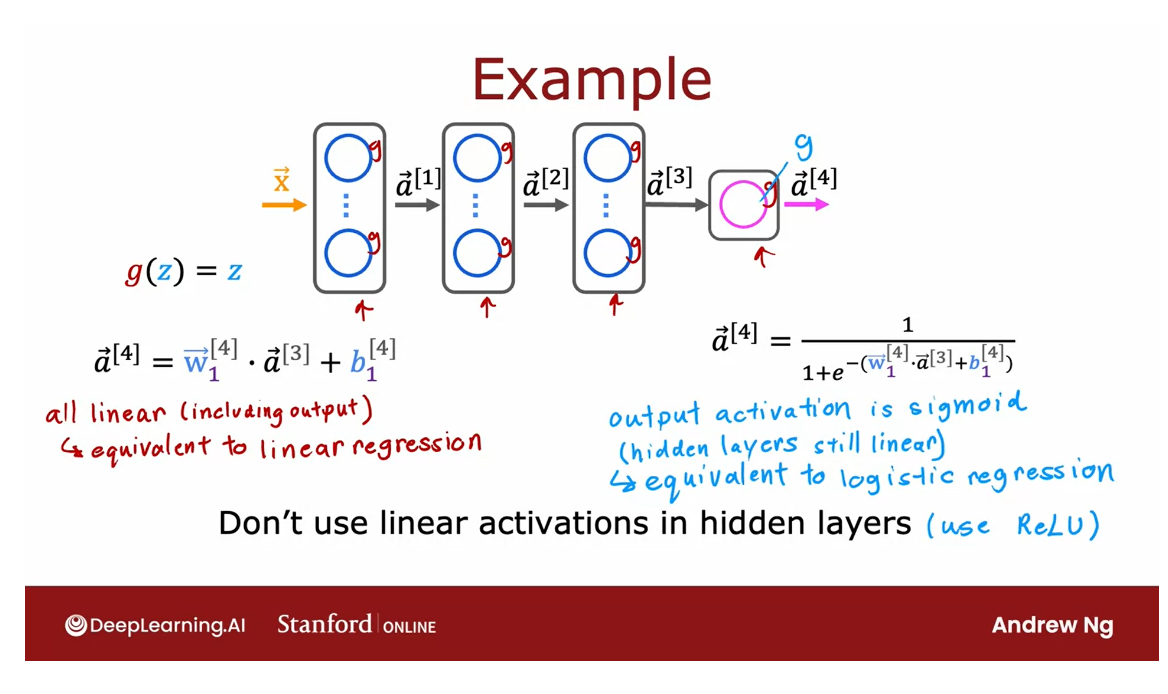
So in the general case, if you had a neural network with multiple layers like this
and say you were to use a linear activation function for all of the hidden layers and also use a linear
activation function for the output layer, then it turns out this
model will compute an output that is completely equivalent to linear regression.
The output a4 can
be expressed as a linear function of the
input features x plus b.
Or alternatively, if we were to still use a linear
activation function for all the hidden layers, for these three
hidden layers here, but we were to use a logistic activation function
for the output layer, then it turns out you
can show that this model becomes equivalent to
logistic regression, and a4, in this case, can be expressed as
1 over 1 plus e to the negative wx plus b for
some values of w and b.
So this big neural network
doesn’t do anything that you can’t also do
with logistic regression.
That’s why a common rule
of thumb is don’t use the linear activation function in the hidden layers
of the neural network.
In fact, I recommend
typically using the ReLU activation function
should do just fine.So that’s why a
neural network needs activation functions other than just the linear activation
function everywhere.
So far, you’ve learned to
build neural networks for binary classification
problems where y is either zero or one. As well as for regression
problems where y can take negative
or positive values, or maybe just positive
and non-negative values. In the next video, I’d like to share with
you a generalization of what you’ve seen so far
for classification. In particular, when y doesn’t
just take on two values, but may take on three or four or ten or even
more categorical values. Let’s take a look at
how you can build a neural network for that type
of classification problem.
Lab: ReLU activation
Optional Lab - ReLU activation
import numpy as np
import matplotlib.pyplot as plt
from matplotlib.gridspec import GridSpec
plt.style.use('./deeplearning.mplstyle')
import tensorflow as tf
from tensorflow.keras.models import Sequential
from tensorflow.keras.layers import Dense, LeakyReLU
from tensorflow.keras.activations import linear, relu, sigmoid
%matplotlib widget
from matplotlib.widgets import Slider
from lab_utils_common import dlc
from autils import plt_act_trio
from lab_utils_relu import *
import warnings
warnings.simplefilter(action='ignore', category=UserWarning)
2 - ReLU Activation
This week, a new activation was introduced, the Rectified Linear Unit (ReLU).
a = m a x ( 0 , z ) ReLU function a = max(0,z) \quad\quad\text { ReLU function} a=max(0,z) ReLU function
plt_act_trio()
Output
The example from the lecture on the right shows an application of the ReLU. In this example, the derived “awareness” feature is not binary but has a continuous range of values. The sigmoid is best for on/off or binary situations. The ReLU provides a continuous linear relationship. Additionally it has an ‘off’ range where the output is zero.
The “off” feature makes the ReLU a Non-Linear activation. Why is this needed? Let’s examine this below.
Why Non-Linear Activations?
The function shown is composed of linear pieces (piecewise linear). The slope is consistent during the linear portion and then changes abruptly at transition points. At transition points, a new linear function is added which, when added to the existing function, will produce the new slope. The new function is added at transition point but does not contribute to the output prior to that point. The non-linear activation function is responsible for disabling the input prior to and sometimes after the transition points. The following exercise provides a more tangible example.
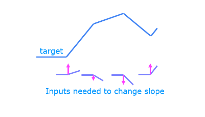
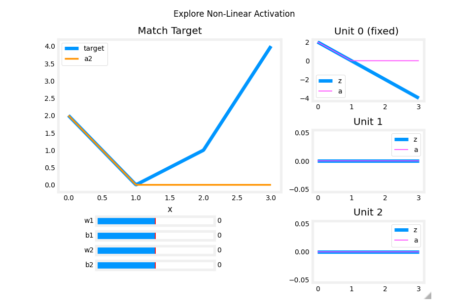
The exercise will use the network below in a regression problem where you must model a piecewise linear target :
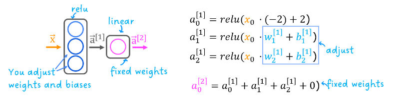
The network has 3 units in the first layer. Each is required to form the target. Unit 0 is pre-programmed and fixed to map the first segment. You will modify weights and biases in unit 1 and 2 to model the 2nd and 3rd segment. The output unit is also fixed and simply sums the outputs of the first layer.
Using the sliders below, modify weights and bias to match the target.
Hints: Start with w1 and b1 and leave w2 and b2 zero until you match the 2nd segment. Clicking rather than sliding is quicker. If you have trouble, don’t worry, the text below will describe this in more detail.
_ = plt_relu_ex()
Output
自己手动调整一下
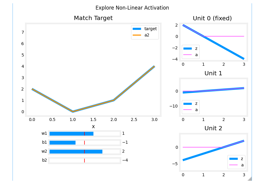
The goal of this exercise is to appreciate how the ReLU’s non-linear behavior provides the needed ability to turn functions off until they are needed. Let’s see how this worked in this example.
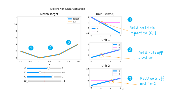
The plots on the right contain the output of the units in the first layer.
Starting at the top, unit 0 is responsible for the first segment marked with a 1. Both the linear function z z z and the function following the ReLU a a a are shown. You can see that the ReLU cuts off the function after the interval [0,1]. This is important as it prevents Unit 0 from interfering with the following segment.
Unit 1 is responsible for the 2nd segment. Here the ReLU kept this unit quiet until after x is 1. Since the first unit is not contributing, the slope for unit 1, w 1 [ 1 ] w^{[1]}_1 w1[1], is just the slope of the target line. The bias must be adjusted to keep the output negative until x has reached 1. Note how the contribution of Unit 1 extends to the 3rd segment as well.
Unit 2 is responsible for the 3rd segment. The ReLU again zeros the output until x reaches the right value.The slope of the unit, w 2 [ 1 ] w^{[1]}_2 w2[1], must be set so that the sum of unit 1 and 2 have the desired slope. The bias is again adjusted to keep the output negative until x has reached 2.
The “off” or disable feature of the ReLU activation enables models to stitch together linear segments to model complex non-linear functions.
[4] Practice quiz: Activation Functions
Practice quiz: Activation Functions
Latest Submission Grade 100%
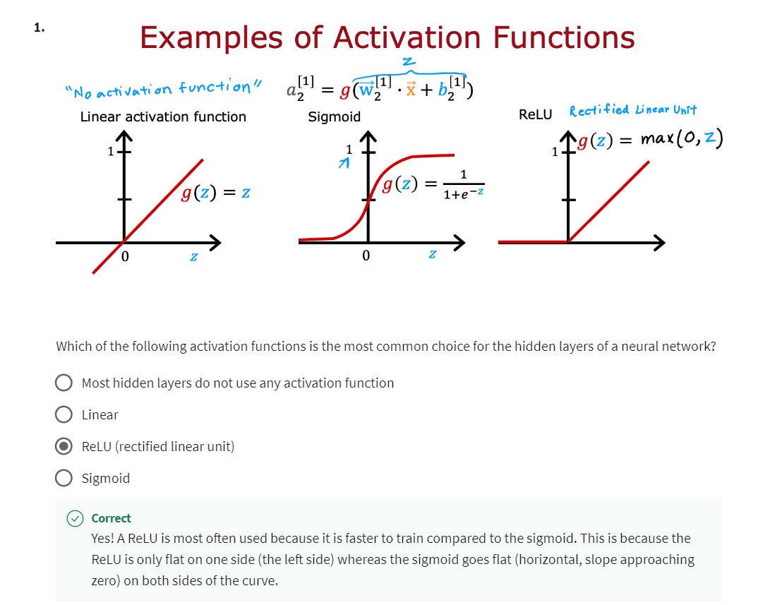
Yes! A ReLU is most often used because it is faster to train compared to the sigmoid. This is because the ReLU is only flat on one side (the left side) whereas the sigmoid goes flat (horizontal, slope approaching zero) on both sides of the curve.
[5] Multiclass Classification
Multiclass
Multiclass classification
Multiclass classification refers
to classification problems where you can have more than just two possible
output labels so not just zero or 1.
Let’s take a look at what that means.
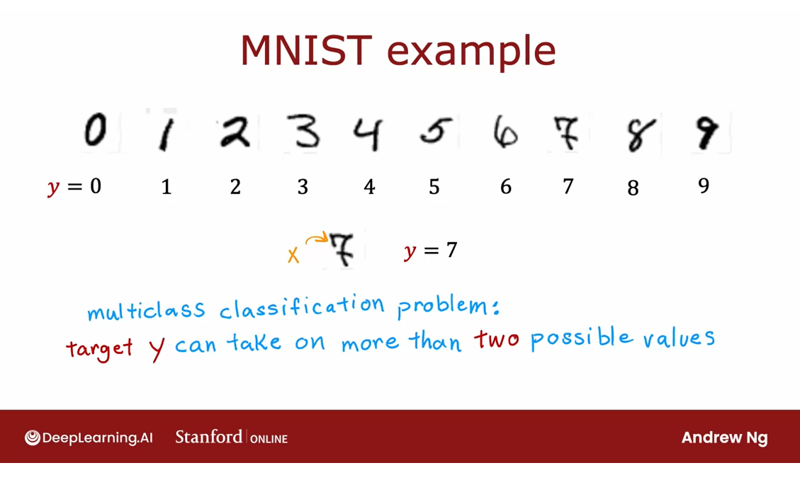
For the handwritten digit classification
problems we’ve looked at so far, we were just trying to distinguish
between the handwritten digits 0 and 1.
But if you’re trying to read protocols or
zip codes in an envelope, well, there are actually 10 possible
digits you might want to recognize.Or alternatively in the first course
you saw the example if you’re trying to classify whether
patients may have any of three or five different possible diseases.
That too would be a multiclass
classification problem or one thing I’ve worked on a lot
is visual defect inspection of parts manufacturer in the factory.Where you might look at the picture
of a pill that a pharmaceutical company has manufactured and
try to figure out does it have a scratch effect or
discoloration defects or a chip defect.
Can be used in pharmaceutical company to classify pills
And this would again be multiple
classes of multiple different types of defects that you could
classify this pill is having.
So a multiclass classification problem is
still a classification problem in that y you can take on only a small number of
discrete categories is not any number, but now y can take on more
than just two possible values.
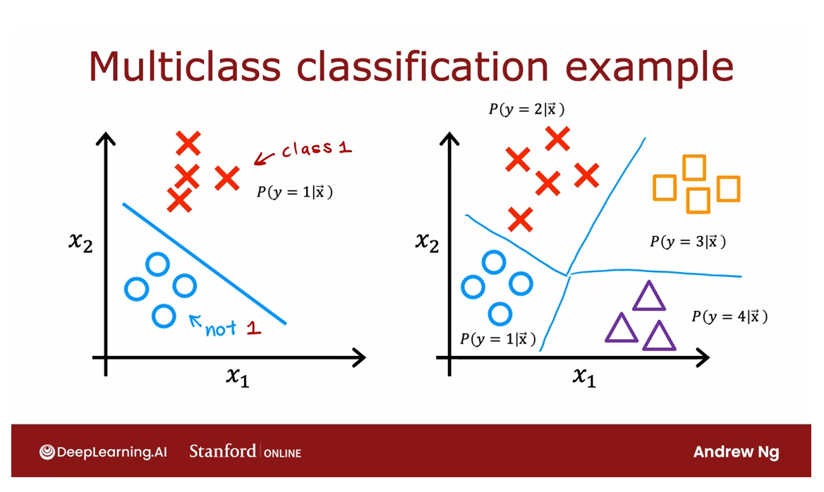
So whereas previously for
buying the classification, you may have had a data set like
this with features x1 and x2. In which case logistic regression
would fit model to estimate what the probability of y being 1,
given the features x.
Because y was either 01 with
multiclass classification problems, you would instead have a data
set that maybe looks like this.
Where we have four classes where
the Os represents one class, the xs represent another class.The triangles represent
the third class and the squares represent the fourth class.
And instead of just estimating
the chance of y being equal to 1, well, now want to estimate what’s
the chance that y is equal to 1, or what’s the chance that y is equal to 2? Or what’s the chance that y is equal to 3,
or the chance of y being equal to 4?
And it turns out that the algorithm you
learned about in the next video can learn a decision boundary that maybe
looks like this that divides the space exploded next to into four categories
rather than just two categories.
So that’s the definition of
the multiclass classification problem.
In the next video, we’ll look at
the softmax regression algorithm which is a generalization of the logistic
regression algorithm and using that you’ll be able to carry out
multiclass classification problems.
And after that we’ll take
softmax regression and fit it into a new neural network so
that you’ll also be able to train a neural network to carry out multiclass
classification problems. Let’s go on to the next video.
Softmax
Numerical stability is improved if the softmax is grouped with the loss function rather than the output layer during training
The softmax regression
algorithm is a generalization of
logistic regression, which is a binary
classification algorithm to the multiclass
classification contexts.
Let’s take a look at how works.
Recall that logistic
regression applies when y can take on two
possible output values, either zero or one, and the way it computes
this output is, you would first
calculate z equals w.product of x plus b, and then you would compute
what I’m going to call here a equals g of z which is a
sigmoid function applied to z.
We interpreted this as logistic
regressions estimates of the probability of
y being equal to 1 given those input features x.Now, quick quiz question; if the probability of
y equals 1 is 0.71, then what is the probability
that y is equal to zero?
Well, the chance of
y being the one, and the chances of
y being the zero, they’ve got to add
up to one, right?So there’s a 71 percent
chance of it being one, there has to be a 29 percent or 0.29 chance of it
being equal to zero.
为了稍微修饰一下logistic回归,为我们建立对softmax回归的推广,我将把logistic回归看作是实际计算两个数字
To embellish logistic
regression a little bit in order to set us up for the generalization to
softmax regression, I’m going to think of logistic
regression as actually computing two numbers: First a_1 which is this quantity
that we had previously of the chance of y being
equal to 1 given x, and second, I’m
going to think of logistic regression as
also computing a_2, which is 1 minus this which is just the chance of y being equal to zero given
the input features x, and so a_1 and a_2, of course, have to add up to 1.
Let’s now generalize this
to softmax regression, and I’m going to do this
with a concrete example of when y can take on
four possible outputs, so y can take on the values 1, 2, 3 or 4.
Here’s what softmax
regression will do, it will compute z_1 as
w_1.product with x plus b_1, and then z_2 equals
w_2.product of x plus b_2, and so on for z_3 and z_4. Here, w_1, w_2, w_3, w_4 as well as b_1, b_2, b_3, b_4, these are the parameters
of softmax regression.
Next, here’s the formula
for softmax regression, we’ll compute a_1 equals
e^z_1 divided by e^ z_1, plus e^ z_2, plus e^z_3 plus, e^ z_4, and a_1 will
be interpreted as the algorithms estimate
of the chance of y being equal to 1 given
the input features x.
Then the formula for
softmax regression, we’ll compute a_2 equals e^ z_2 divided by the
same denominator, e^z_1 plus e^z_2, plus e^z_3, plus e^z4, and we’ll interpret a_2 as
the algorithms estimate of the chance that y is equal to 2 given the input features x.
Similarly for a_3, where here the numerator is now e^z_3 divided by
the same denominator, that’s the estimated
chance of y being a_3, and similarly a_4 takes
on this expression.
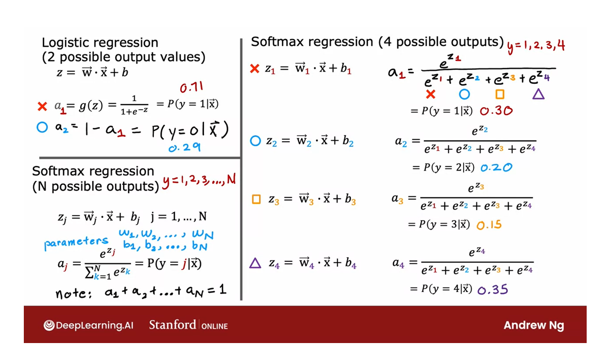
Cost
Whereas on the left, we wrote down the specification for the logistic
regression model, these equations on the right are our specification for the
softmax regression model.It has parameters
w_1 through w_4, and b_1 through b_4, and if you can learn appropriate choices to
all these parameters, then this gives you a way of predicting what’s the
chance of y being 1, 2, 3 or 4, given a set of input features x.
Quick quiz, let’s see, run softmax regression
on a new input x, and you find that a_1 is 0.30, a_2 is 0.20, a_3 is 0.15. What do you think a_4 will be? Why don’t you take a look
at this quiz and see if you can figure out
the right answer?
You might have
realized that because the chance of y take
on the values of 1, 2, 3 or 4, they have
to add up to one, a_4 the chance of y being
with a four has to be 0.35, which is 1 minus 0.3
minus 0.2 minus 0.15.
Here I wrote down
the formulas for softmax regression in the case
of four possible outputs, and let’s now write
down the formula for the general case for
softmax regression.
In the general case
In the general case, y can take on n possible values, so y can be 1, 2, 3, and so on up to n.
In that case, softmax regression
will compute to z_ j equals w_ j.product
with x plus b_j, where now the parameters of
softmax regression are w_1, w_2 through to w_n, as well as b_1, b_2 through b_n.
Then finally, we’ll
compute a j equals e to the z j divided
by sum from k equals 1 to n of e to the z sub
k.
While here I’m using another variable k to index
the summation because here j refers to a specific
fixed number like j equals 1. A, j is interpreted as the model’s estimate that y is equal to j given the
input features x.
Notice that by construction
that this formula, if you add up a1, a2 all the way through a n, these numbers always will
end up adding up to 1.
We specified how you would compute the softmax
regression model. I won’t prove it in this video, but it turns out
that if you apply softmax regression
with n equals 2, so there are only two
possible output classes then softmax regression ends up computing basically the same thing as logistic regression.
Softmax regression can be reduced to logistic regression
The parameters end up being
a little bit different, but it ends up reducing to
logistic regression model.
But that’s why the
softmax regression model is the generalization
of logistic regression.
Having defined how
softmax regression computes it’s outputs, let’s now take a look at how to specify the cost function
for softmax regression.
Recall for logistic regression,
this is what we had. We said z is equal to this. Then I wrote earlier
that a1 is g of z, was interpreted as a
probability of y is 1.We also wrote a2 is the
probability that y is equal to 0. Previously, we had written the loss of logistic
regression as negative y log a1 minus 1
minus y log 1 minus a1.
But 1 minus a1 is
also equal to a2, because a2 is one minus a1 according to this
expression over here.
I can rewrite or
simplify the loss for logistic regression
little bit to be negative y log a1 minus
1 minus y log of a2.In other words, the
loss if y is equal to 1 is negative log a1. If y is equal to 0, then the
loss is negative log a2, and then same as before
the cost function for all the parameters in the
model is the average loss, average over the
entire training set.
That was a cost function
for this regression.
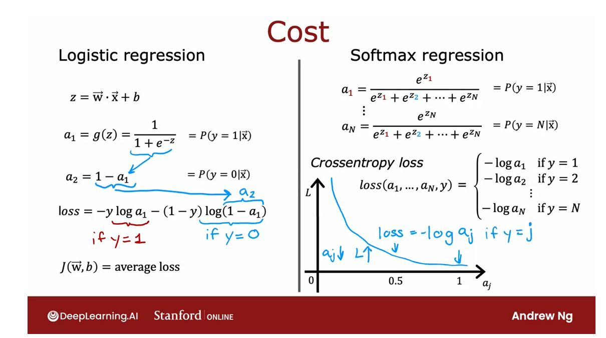
Let’s write down the
cost function that is conventionally use
the softmax regression.Recall that these
are the equations we use for softmax regression.
The loss we’re going to use for softmax regression is just this. The loss for if the algorithm
puts a1 through an.The ground truth label
is why is if y equals 1, the loss is negative log a1. Says negative log of
the probability that it thought y was equal to 1, or if y is equal to 2, then I’m going to define
as negative log a2. Y is equal to 2.
The loss of the algorithm
on this example is negative log of the probability it’s
thought y was equal to 2. On all the way down to
if y is equal to n, then the loss is negative log of a n.
To illustrate
what this is doing, if y is equal to j, then the loss is
negative log of a j. That’s what this
function looks like. Negative log of a j is a
curve that looks like this. If a j was very close to 1, then you beyond this part of the curve and the loss
will be very small.
But if it thought, say, a j had only a 50% chance then the loss gets a
little bit bigger. The smaller a j is, the bigger the loss. This incentivizes
the algorithm to make a j as large as possible, as close to 1 as possible.Because whatever the
actual value y was, you want the algorithm to say hopefully that the chance of y being that value
was pretty large.
Notice that in this
loss function, y in each training example
can take on only one value. You end up computing
this negative log of a j only for one value of a j, which is whatever was
the actual value of y equals j in that
particular training example.For example, if y
was equal to 2, you end up computing
negative log of a2, but not any of the
other negative log of a1 or the other terms here.
That’s the form of
the model as well as the cost function for
softmax regression. If you were to train this model, you can start to build multiclass classification
algorithms.
What we’d like to do next is take this softmax
regression model, and fit it into a new network so that you really do
something even better, which is to train a new network for
multi-class classification. Let’s go through that
in the next video.
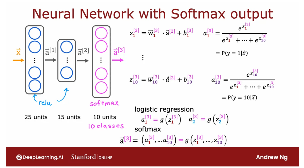
Neural Network with Softmax output
In order to build a Neural Network that
can carry out multi class classification, we’re going to take the Softmax
regression model and put it into essentially the output
layer of a Neural Network.Let’s take a look at how to do that.
Previously, when we were doing handwritten
digit recognition with just two classes. We use a new Neural Network
with this architecture.
Do handwritten digit classification with 10 classes: have 10 output units
If you now want to do handwritten
digit classification with 10 classes, all the digits from zero to nine,
then we’re going to change this Neural Network to have
10 output units like so.And this new output layer will
be a Softmax output layer.
Has a softmax output / softmax layer
So sometimes we’ll say this
Neural Network has a Softmax output or that this upper layer is a Softmax layer.
And the way forward propagation
works in this Neural Network is given an input X A1 gets computed
exactly the same as before.And then A2, the activations for the second hidden layer also get
computed exactly the same as before.
And we now have to compute the activations
for this output layer, that is a3. This is how it works.
If you have 10 optical classes,
we will compute Z1, Z2 through Z10 using these expressions.So this is actually very similar
to what we had previously for the formula you’re using to compute Z. Z1 is W1.product with a2,
the activations from the previous layer plus b1 and
so on for Z1 through Z10.Then a1 is equal to e to the Z1 divided by e to the Z1 plus up to e to the Z10.
And that’s our estimate of
the chance that y is equal to 1. And similarly for a2 and
similarly all the way up to a10.
And so this gives you your estimates
of the chance of y being good to one, two and so on up through
the 10th possible label for y. And just for completeness, if you want to indicate that these are the
quantities associated with layer three, technically, I should add these
super strip three’s there.
It does make the notation
a little bit more cluttered.But this makes explicit that this is,
for example, the Z(3), 1 value and
this is the parameters associated with the first unit of layer
three of this Neural Network.And with this, your Softmax open
layer now gives you estimates of the chance of y being any of
these 10 possible output labels.
I do want to mention that the Softmax
layer will sometimes also called the Softmax activation function,
it is a little bit unusual in one respect compared to the other
activation functions we’ve seen so far, like sigmoid, radial and
linear, which is that when we’re looking at sigmoid or value or
linear activation functions, a1 was a function of Z1 and
a2 was a function of Z2 and only Z2.
In other words,
to obtain the activation values, we could apply the activation
function g be it sigmoid or rarely or something else element wise to Z1 and Z2
and so on to get a1 and a2 and a3 and a4.
But with the Softmax activation function, notice that a1 is a function of Z1 and
Z2 and Z3 all the way up to Z10.So each of these activation values,
it depends on all of the values of Z. And this is a property that’s a bit
unique to the Softmax output or the Softmax activation function or stated differently if you want
to compute a1 through a10,hat is a function of Z1 all the way
up to Z 10 simultaneously.
And this is unlike the other
activation functions we’ve seen so far.
How to implement in TensorFlow?
Finally, let’s look at how you
would implement this in tensorflow.If you want to implement the neural
network that I’ve shown here on this slide, this is the code to do so. Similar as before there are three steps
to specifying and training the model.
The first step is to tell tensorflow to
sequentially string together three layers. First layer, is this 25 units with
rail you activation function. Second layer,
15 units of rally activation function. And then the third layer,
because there are now 10 output units, you want to output a1 through a10,
so they’re now 10 output units.
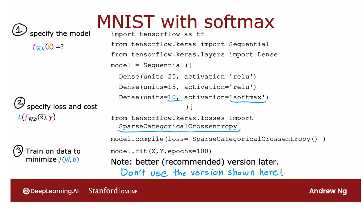
Cost function: SparseCategoricalCrossentropy
And we’ll tell tensorflow to use
the Softmax activation function.And the cost function that
you saw in the last video, tensorflow calls that the
SparseCategoricalCrossentropy function. So I know this name is a bit
of a mouthful, whereas for logistic regression we had
the BinaryCrossentropy function, here we’re using the
SparseCategoricalCrossentropy function.
And what sparse categorical refers to is that you’re still
classified y into categories. So it’s categorical. This takes on values from 1 to 10.
Sparce refers to that y can only take on one of these values.
Refers to each output is only one of these categories.
And sparse refers to that y can only
take on one of these 10 values. So each image is either 0 or
1 or 2 or so on up to 9.You’re not going to see a picture that
is simultaneously the number two and the number seven so sparse refers to that each digit
is only one of these categories.
But so that’s why the loss function
that you saw in the last video, it’s called intensive though the sparse
categorical cross entropy loss function.
And then the code for training
the model is just the same as before.And if you use this code, you can train a neural network on
a multi class classification problem.
Just one important note, if you use this
code exactly as I’ve written here, it will work, but don’t actually use this code
because it turns out that in tensorflow, there’s a better version of the code
that makes tensorflow work better.
So even though the code
shown in this slide works. Don’t use this code the way
I’ve written it here, because in a later video this week
you see a different version that’s actually the recommended version of
implementing this, that will work better.But we’ll take a look at
that in a later video.
So now, you know how to train a neural
network with a softmax output layer with one caveat.
There’s a different version of
the code that will make tensorflow able to compute these
probabilities much more accurately. Let’s take a look at that in the next
video, we should also show you the actual code that I recommend you use if you’re
training a Softmax neural network. Let’s go on to the next video.
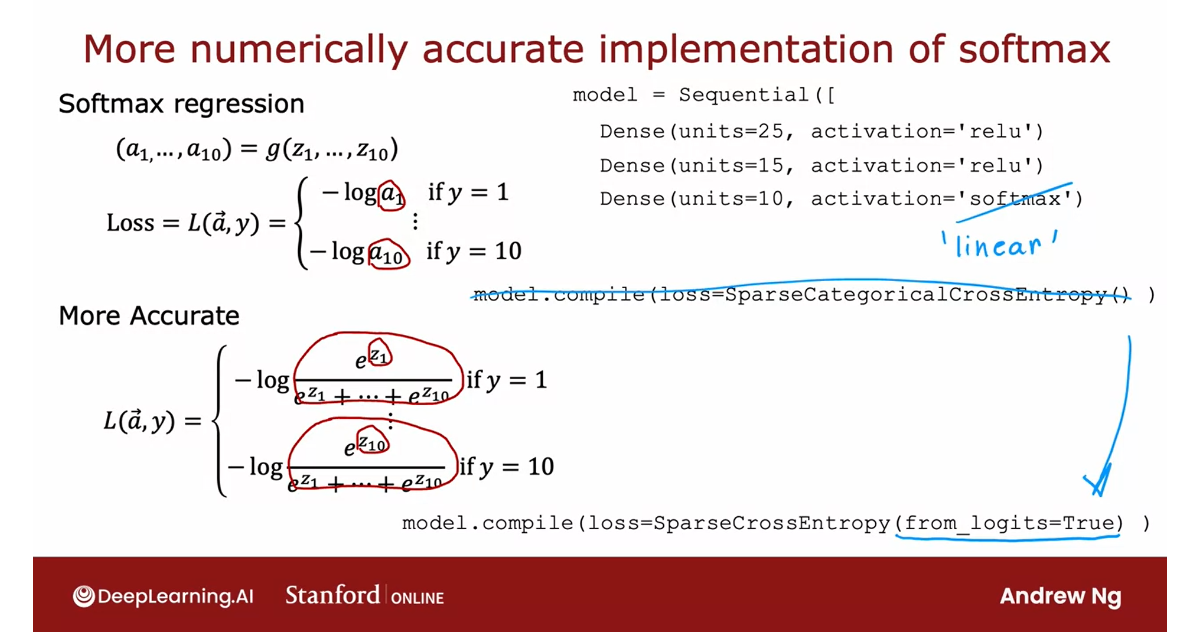
Improved implementation of softmax
Numerical Roundoff Errors
The implementation that you
saw in the last video of a neural network with a
softmax layer will work okay.But there’s an even better
way to implement it. Let’s take a look at
what can go wrong with that implementation and
also how to make it better.
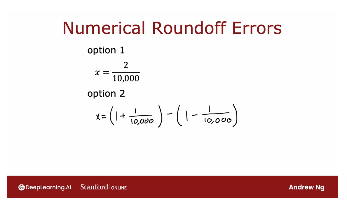
Two different ways of computing the same quantity
Let me show you two
different ways of computing the same
quantity in a computer.
Option 1, we can set
x equals to 2/10,000.
Option 2, we can set x equals 1 plus 1/10,000 minus
1 minus 1/10,000, which you first compute this, and then compute this, and
you take the difference.If you simplify this expression, this turns out to be
equal to 2/10,000.
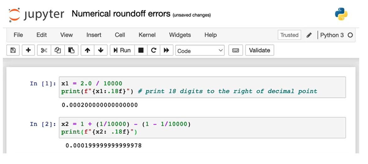
Print the result to a lot of decimal points of accuracy
Let me illustrate this
in this notebook.First, let’s set x equals
2/10,000 and print the result to a lot of decimal points of accuracy.
That looks pretty good.Second, let me set x equals, I’m going to insist
on computing 1/1 plus 10,000 and then subtract
from that 1 minus 1/10,000.Let’s print that out.
It just looks a little bit off this as if there’s
some round-off error.
Only a finite amount of memory to store a number
The result can have more or less numerical round-off error
Because the computer has only a finite amount of
memory to store each number, called a floating-point
number in this case, depending on how you decide to compute the value 2/10,000, the result can have more or less numerical round-off error.
Reduce numerical round-off errors, leading to more accurate computations
It turns out that while
the way we have been computing the cost function
for softmax is correct, there’s a different way
of formulating it that reduces these numerical
round-off errors, leading to more accurate
computations within TensorFlow.
Let me first explain this a little bit more detail
using logistic regression.Then we will show how
these ideas apply to improving our
implementation of softmax.
First, let me illustrate these ideas using
logistic regression. Then we’ll move on to
show how to improve your implementation
of softmax as well.
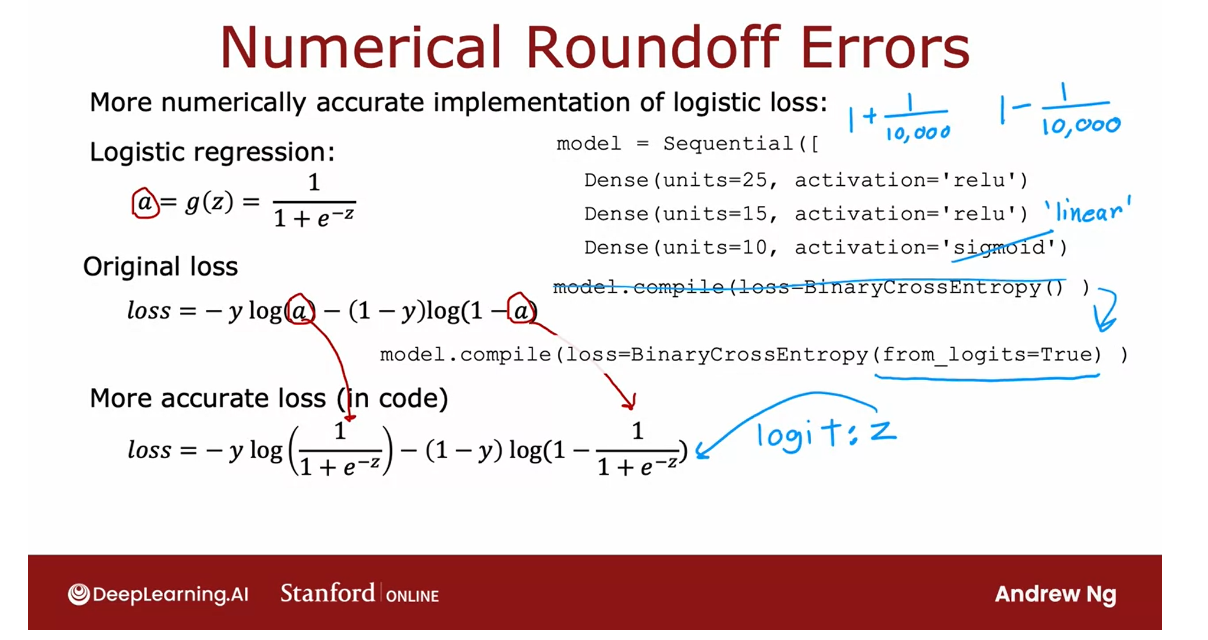
Recall that for
logistic regression, if you want to compute the loss function
for a given example, you would first compute
this output activation a, which is g of z or 1/1
plus e to the negative z.Then you will compute the loss using this expression over here.
In fact, this is what the
codes would look like for a logistic output layer with this binary cross entropy loss.
For logistic regression,
this works okay, and usually the numerical round-off errors
aren’t that bad.
Compute a number as an intermediate value
But it turns out
that if you allow TensorFlow to not have to compute a as an
intermediate term. But instead, if you
tell TensorFlow that the loss this
expression down here.All I’ve done is I’ve
taken a and expanded it into this
expression down here.
Then TensorFlow can rearrange terms in this expression and come up with a more
numerically accurate way to compute this loss function.Whereas the original
procedure was like insisting on computing as
an intermediate value, 1 plus 1/10,000 and another
intermediate value, 1 minus 1/10,000, t hen manipulating these
two to get 2/10,000.
This artial implementation
was insisting on explicitly computing a as an
intermediate quantity.
But instead, by specifying this expression at the bottom directly as the loss function, it gives TensorFlow more
flexibility in terms of how to compute this
and whether or not it wants to compute
a explicitly.
The code you can use to do this is shown here and
what this does is it sets the output
layer to just use a linear activation
function and it puts both the
activation function, 1/1 plus to the negative z, as well as this cross
entropy loss into the specification of the
loss function over here.
from_logits = True
logits: z
make computation more accurately
That’s what this from logits equals true argument
causes TensorFlow to do.In case you’re wondering
what the logits are, it’s basically this
number z. TensorFlow will compute z as an
intermediate value, but it can rearrange
terms to make this become computed
more accurately.
Downside: code becomes less legible
One downside of this code is it becomes a little
bit less legible. But this causes TensorFlow to have a little bit less
numerical roundoff error.
Now in the case of
logistic regression, either of these implementations
actually works okay, but the numerical
roundoff errors can get worse when it comes to softmax.
When it comes to softmax, the numerical roundoff errors can get worse
Now let’s take this idea and
apply to softmax regression. Recall what you saw
in the last video was you compute the
activations as follows.
The activations is g of z_1, through z_10 where
a_1, for example, is e to the z_1 divided by the sum of the e to the z_j’s, and then the loss was
this depending on what is the actual value of y
is negative log of aj for one of the aj’s
and so this was the code that we had to do this computation in
two separate steps.
Give TensorFlow the ability to rearrange terms and compute this integral numerically accurate way.
But once again, if
you instead specify that the loss is
if y is equal to 1 is negative log of
this formula, and so on. If y is equal to 10
is this formula, then this gives
TensorFlow the ability to rearrange terms and compute this integral numerically
accurate way.
TensorFlow can avoid some of very small or very large numbers
Come up with more accurate computation for the loss function
Just to give you
some intuition for why TensorFlow might
want to do this, it turns out if one
of the z’s really small than e to negative
small number becomes very, very small or if one of the
z’s is a very large number, then e to the z can become a very large number and
by rearranging terms,
TensorFlow can avoid some of these very small or
very large numbers and therefore come up with more accurate computation
for the loss function.
The code for doing this is shown here in the output layer, we’re now just using a linear
activation function so the output layer just
computes z_1 through z_10 and this whole computation of the loss is then captured in
the loss function over here, where again we have
the from_logists equals true parameter.
Once again, these two pieces of code do pretty much
the same thing, except that the version that is recommended is more
numerically accurate, although unfortunately, it is a little bit harder
to read as well.
If you’re reading
someone else’s code and you see this and
you’re wondering what’s going on is actually equivalent to the
original implementation, at least in concept, except that is more
numerically accurate.
The numerical roundoff
errors for_logist regression aren’t that bad, but it is recommended
that you use this implementation down to the bottom instead,
and conceptually, this code does the same thing as the first version that
you had previously, except that it is a little bit
more numerically accurate.
Although the downside is maybe just a little bit harder
to interpret as well.
The NN’s final layer no longer outputs probabilities a 1 a_{1} a1 to a 10 a_{10} a10
It is instead of putting z 1 z_{1} z1 through z 10 z_{10} z10
Now there’s just
one more detail, which is that we’ve now changed
the neural network to use a linear activation function rather than a softmax
activation function.The neural network’s
final layer no longer outputs these
probabilities A_1 through A_10. It is instead of putting
z_1 through z_10.
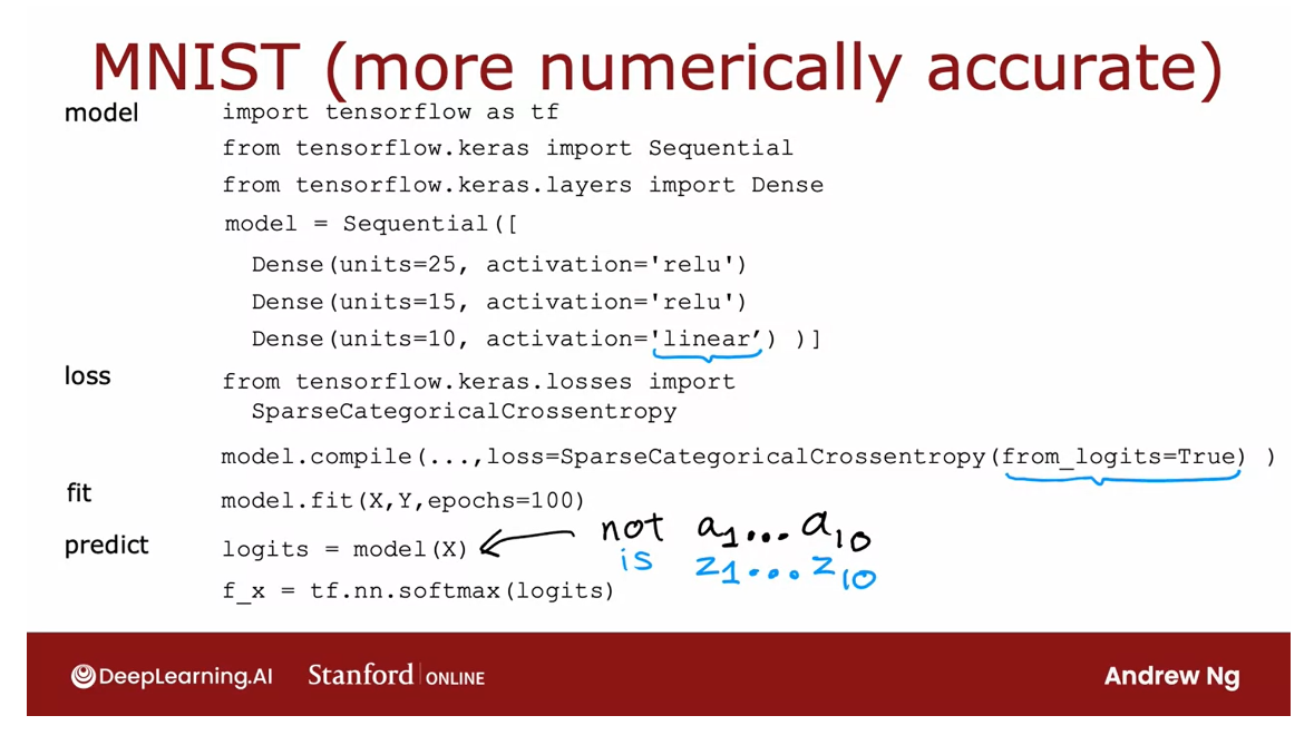
Logistic regression
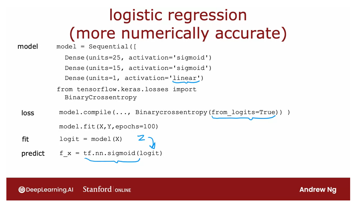
Here’s the code again for the
neural network where we had the model with now the
linear activation in the output layer and then
also this new loss function.
After you’ve trained the model, when you’re actually
making a prediction, please be aware that if
you were to calculate predictions equals model
applied to say a new example X, these predictions are no
longer A_1 through A_10. The probabilities
that you might want.
Need to apply to softmax function to z 1 z_{1} z1 through z 10 z_{10} z10
These are instead z_1 through Z_10 and so if you wants
to get the probabilities, you still have to take these numbers z_1
through z_10 and apply the softmax function
to them and that’s what will actually get
you, the probabilities.
I didn’t talk about it in the case of logistic regression, but if you were combining the output’s logistic function
with the loss function, then for logistic regressions, you also have to change the code this way to take
the output value and map it through the logistic function in order to actually get the probability.
You now know how to do
multi-class classification with a softmax output layer and also how to do it in a
numerically stable way.
Before wrapping up
multi-class classification, I want to share with
you one other type of classification problem called a multi-label
classification problem. Let’s talk about that
in the next video.
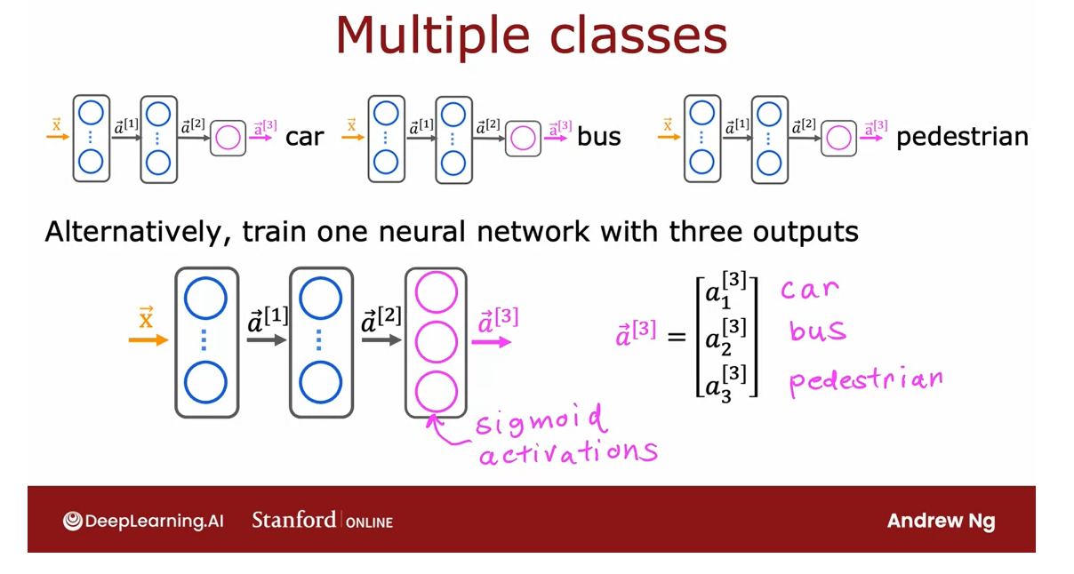
Classification with multiple outputs (Optional)
Multi label Classification
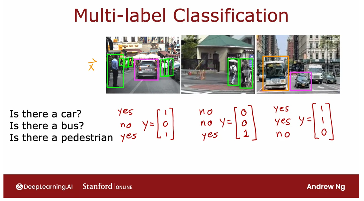
You’ve learned about
multi-class classification, where the output label
Y can be any one of two or potentially many more than two possible categories.
There’s a different type of classification problem called a multi-label
classification problem, which is where associate
of each image, they could be multiple labels. Let me show you what
I mean by that.
If you’re building a
self-driving car or maybe a driver
assistance system, then given a picture of
what’s in front of your car, you may want to ask
a question like, is there a car or
at least one car? Or is there a bus, or is there a pedestrian or
are there any pedestrians?
In this case, there is a car, there is no bus, and there is at
least one pedestrian or in this second
image, no cars, no buses and yes to
pedestrians and yes car, yes bus and no pedestrians.
These are examples of multi-label classification
problems because associated with a single input, image X are three
different labels corresponding to whether
or not there are any cars, buses, or pedestrians
in the image.
The target of Y is actually a vector of three numbers
In this case, the
target of the Y is actually a vector
of three numbers, and this is as distinct from multi-class
classification, where for, say handwritten digit
classification, Y was just a single number, even if that number
could take on 10 different possible values.
| Multi-class classification | Multi-label classification |
|---|---|
| Output label y can be any one of many possible categories | Output label can be a vector of many numbers |
How to build a neural network for multi-label classification
How do you build a
neural network for multi-label classification? One way to go about it
is to just treat this as three completely separate
machine learning problems.
You could build
one neural network to decide, are there any cars? The second one to
detect buses and the third one to
detect pedestrians. That’s actually not an
unreasonable approach.Here’s the first neural
network to detect cars, second one to detect buses, third one to detect pedestrians.
Train a single NN to simultaneously detect all three of cars, buses, and pedestrians
But there’s another
way to do this, which is to train a
single neural network to simultaneously detect
all three of cars, buses, and
pedestrians, which is, if your neural
network architecture, looks like this,
there’s input X.
First hidden layer offers a^1, second hidden layer offers a^2, and then the final output
layer, in this case, we’ll have three output
neurals and we’ll output a^3, which is going to be a
vector of three numbers.
Because we’re solving three binary classification
problems, so is there a car? Is there a bus? Is
there a pedestrian? You can use a sigmoid
activation function for each of these three nodes in
the output layer, and so a^3 in this
case will be a_1^3, a_2^3, and a_3^3, corresponding to whether
or not the learning [inaudible] as a car and no bus, and no pedestrians in the image.
Confused wit each other
Multi-class classification and
multi-label classification are sometimes confused
with each other, and that’s why in this video
I want to share with you just a definition of multi-label classification
problems as well, so that depending on
your application, you could choose the right one for the job you want to do.
So that’s it for
multi-label classification. I find that sometimes
multi-class classification and multi-label classification
are confused with other, which is why I wanted
to expressively, in this video,
share with you what is multi-label classification, so that depending on
your application you can choose to write to for
the job that you want to do.And that wraps up the section on multi-class and multi-label
classification.
In the next video,
we’ll start to look at some more advanced
neural network concepts, including an
optimization algorithm that is even better
than gradient descent. Let’s take a look at that
algorithm in the next video, because it’ll help you to get your learning algorithms
to learn much faster. Let’s go on to the next video.
Lab: Softmax
Optional Lab - Softmax Function
In this lab, we will explore the softmax function. This function is used in both Softmax Regression and in Neural Networks when solving Multiclass Classification problems.
import numpy as np
import matplotlib.pyplot as plt
plt.style.use('./deeplearning.mplstyle')
import tensorflow as tf
from tensorflow.keras.models import Sequential
from tensorflow.keras.layers import Dense
from IPython.display import display, Markdown, Latex
from sklearn.datasets import make_blobs
%matplotlib widget
from matplotlib.widgets import Slider
from lab_utils_common import dlc
from lab_utils_softmax import plt_softmax
import logging
logging.getLogger("tensorflow").setLevel(logging.ERROR)
tf.autograph.set_verbosity(0)
Note: Normally, in this course, the notebooks use the convention of starting counts with 0 and ending with N-1, ∑ i = 0 N − 1 \sum_{i=0}^{N-1} ∑i=0N−1, while lectures start with 1 and end with N, ∑ i = 1 N \sum_{i=1}^{N} ∑i=1N. This is because code will typically start iteration with 0 while in lecture, counting 1 to N leads to cleaner, more succinct equations. This notebook has more equations than is typical for a lab and thus will break with the convention and will count 1 to N.
Softmax Function
In both softmax regression and neural networks with Softmax outputs, N outputs are generated and one output is selected as the predicted category. In both cases a vector z \mathbf{z} z is generated by a linear function which is applied to a softmax function. The softmax function converts z \mathbf{z} z into a probability distribution as described below. After applying softmax, each output will be between 0 and 1 and the outputs will add to 1, so that they can be interpreted as probabilities. The larger inputs will correspond to larger output probabilities.
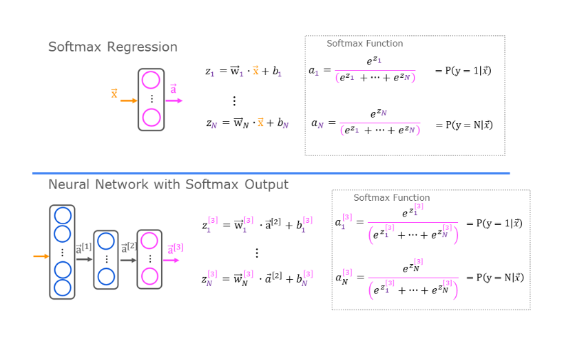
The softmax function can be written:
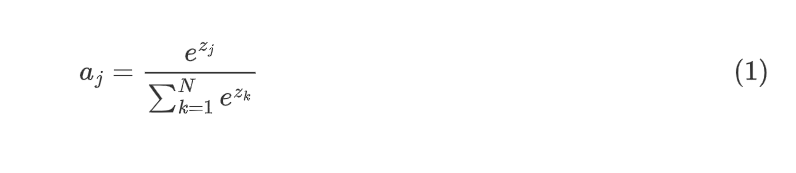
公式render不出来,需要latex语法的见下面代码
\begin{align} a_j = \frac{e^{z_j}}{ \sum_{k=1}^{N}{e^{z_k} }} \tag{1} \end{align}
The output a a a is a vector of length N, so for softmax regression, you could also write:
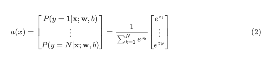
公式render不出来,需要latex语法的见下面代码
\begin{align}
a(x) =
\begin{bmatrix}
P(y = 1 | \mathbf{x}; \mathbf{w},b) \\
\vdots \\
P(y = N | \mathbf{x}; \mathbf{w},b)
\end{bmatrix}
=
\frac{1}{ \sum_{k=1}^{N}{e^{z_k} }}
\begin{bmatrix}
e^{z_1} \\
\vdots \\
e^{z_{N}} \\
\end{bmatrix} \tag{2}
\end{align}
Which shows the output is a vector of probabilities. The first entry is the probability the input is the first category given the input x \mathbf{x} x and parameters w \mathbf{w} w and b \mathbf{b} b.
Let’s create a NumPy implementation:
def my_softmax(z):ez = np.exp(z) #element-wise exponenialsm = ez/np.sum(ez)return(sm)
Below, vary the values of the z inputs using the sliders.
plt.close("all")
plt_softmax(my_softmax)
Output
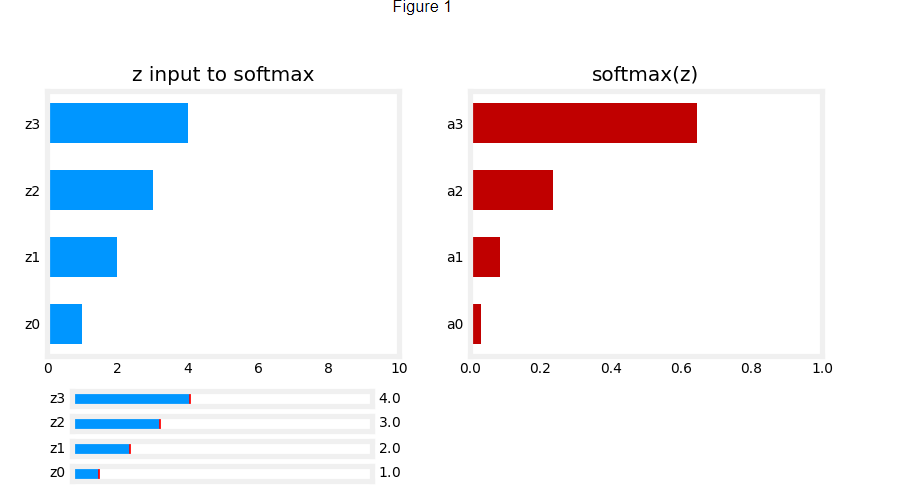
Softmax 改变一个输入,所有的输出都会改变
As you are varying the values of the z’s above, there are a few things to note:
- the exponential in the numerator of the softmax magnifies small differences in the values
- the output values sum to one
- the softmax spans all of the outputs. A change in
z0for example will change the values ofa0-a3. Compare this to other activations such as ReLU or Sigmoid which have a single input and single output.
Cost
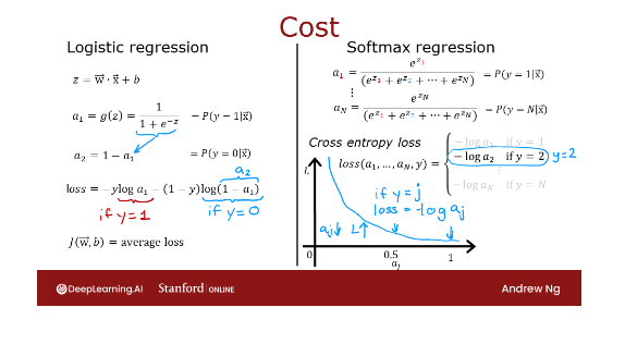
Loss function L
The loss function associated with Softmax, the cross-entropy loss, is:
L ( a , y ) = { − l o g ( a 1 ) , if y = 1 . ⋮ − l o g ( a N ) , if y = N \begin{equation} L(\mathbf{a},y)=\begin{cases} -log(a_1), & \text{if $y=1$}.\\ &\vdots\\ -log(a_N), & \text{if $y=N$} \end{cases} \tag{3} \end{equation} L(a,y)=⎩ ⎨ ⎧−log(a1),−log(aN),if y=1.⋮if y=N(3)
Where y is the target category for this example and a \mathbf{a} a is the output of a softmax function. In particular, the values in a \mathbf{a} a are probabilities that sum to one.
Recall: In this course, Loss is for one example while Cost covers all examples.
Note in (3) above, only the line that corresponds to the target contributes to the loss, other lines are zero.
Cost function J
To write the cost equation we need an ‘indicator function’ that will be 1 when the index matches the target and zero otherwise.
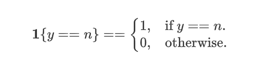
公式render不出来,需要latex语法的见下面代码
\mathbf{1}\{y == n\} = =\begin{cases}1, & \text{if $y==n$}.\\0, & \text{otherwise}.\end{cases}
Now the cost is:
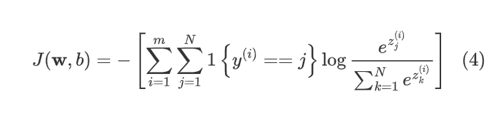
公式render不出来,需要latex语法的见下面代码
\begin{align}
J(\mathbf{w},b) = - \left[ \sum_{i=1}^{m} \sum_{j=1}^{N}  1\left\{y^{(i)} == j\right\} \log \frac{e^{z^{(i)}_j}}{\sum_{k=1}^N e^{z^{(i)}_k} }\right] \tag{4}
\end{align}
Where m m m is the number of examples, N N N is the number of outputs. This is the average of all the losses.
Tensorflow
This lab will discuss two ways of implementing the softmax, cross-entropy loss in Tensorflow, the ‘obvious’ method and the ‘preferred’ method. The former is the most straightforward while the latter is more numerically stable.
Let’s start by creating a dataset to train a multiclass classification model.
# make  dataset for example
centers = [[-5, 2], [-2, -2], [1, 2], [5, -2]]
X_train, y_train = make_blobs(n_samples=2000, centers=centers, cluster_std=1.0,random_state=30)
The Obvious organization
The model below is implemented with the softmax as an activation in the final Dense layer.
The loss function is separately specified in the compile directive.
The loss function is SparseCategoricalCrossentropy. This loss is described in (3) above. In this model, the softmax takes place in the last layer. The loss function takes in the softmax output which is a vector of probabilities.
model = Sequential([ Dense(25, activation = 'relu'),Dense(15, activation = 'relu'),Dense(4, activation = 'softmax')    # < softmax activation here]
)
model.compile(loss=tf.keras.losses.SparseCategoricalCrossentropy(),optimizer=tf.keras.optimizers.Adam(0.001),
)model.fit(X_train,y_train,epochs=10
)
Output
Epoch 1/10
63/63 [==============================] - 0s 941us/step - loss: 0.8368
Epoch 2/10
63/63 [==============================] - 0s 1ms/step - loss: 0.3037
Epoch 3/10
63/63 [==============================] - 0s 1ms/step - loss: 0.1369
Epoch 4/10
63/63 [==============================] - 0s 962us/step - loss: 0.0856
Epoch 5/10
63/63 [==============================] - 0s 1ms/step - loss: 0.0665
Epoch 6/10
63/63 [==============================] - 0s 1ms/step - loss: 0.0566
Epoch 7/10
63/63 [==============================] - 0s 1ms/step - loss: 0.0503
Epoch 8/10
63/63 [==============================] - 0s 990us/step - loss: 0.0455
Epoch 9/10
63/63 [==============================] - 0s 1ms/step - loss: 0.0420
Epoch 10/10
63/63 [==============================] - 0s 1ms/step - loss: 0.0385
Because the softmax is integrated into the output layer, the output is a vector of probabilities.
p_nonpreferred = model.predict(X_train)
print(p_nonpreferred [:2])
print("largest value", np.max(p_nonpreferred), "smallest value", np.min(p_nonpreferred))
Output
[[3.22e-03 3.23e-03 9.65e-01 2.82e-02][9.96e-01 4.10e-03 3.06e-04 1.39e-05]]
largest value 0.99999523 smallest value 8.685352e-10
Preferred
Recall from lecture, more stable and accurate results can be obtained if the softmax and loss are combined during training. This is enabled by the ‘preferred’ organization shown here.
In the preferred organization the final layer has a linear activation. For historical reasons, the outputs in this form are referred to as logits. The loss function has an additional argument: from_logits = True. This informs the loss function that the softmax operation should be included in the loss calculation. This allows for an optimized implementation.
preferred_model = Sequential([ Dense(25, activation = 'relu'),Dense(15, activation = 'relu'),Dense(4, activation = 'linear')   #<-- Note]
)
preferred_model.compile(loss=tf.keras.losses.SparseCategoricalCrossentropy(from_logits=True),  #<-- Noteoptimizer=tf.keras.optimizers.Adam(0.001),
)preferred_model.fit(X_train,y_train,epochs=10
)
Output
Epoch 1/10
63/63 [==============================] - 0s 1ms/step - loss: 0.9501
Epoch 2/10
63/63 [==============================] - 0s 980us/step - loss: 0.4234
Epoch 3/10
63/63 [==============================] - 0s 1ms/step - loss: 0.2043
Epoch 4/10
63/63 [==============================] - 0s 1ms/step - loss: 0.1183
Epoch 5/10
63/63 [==============================] - 0s 1ms/step - loss: 0.0842
Epoch 6/10
63/63 [==============================] - 0s 962us/step - loss: 0.0683
Epoch 7/10
63/63 [==============================] - 0s 1ms/step - loss: 0.0592
Epoch 8/10
63/63 [==============================] - 0s 1ms/step - loss: 0.0530
Epoch 9/10
63/63 [==============================] - 0s 1ms/step - loss: 0.0489
Epoch 10/10
63/63 [==============================] - 0s 945us/step - loss: 0.0452
Output Handling
Notice that in the preferred model, the outputs are not probabilities, but can range from large negative numbers to large positive numbers. The output must be sent through a softmax when performing a prediction that expects a probability.
Let’s look at the preferred model outputs:
p_preferred = preferred_model.predict(X_train)
print(f"two example output vectors:\n {p_preferred[:2]}")
print("largest value", np.max(p_preferred), "smallest value", np.min(p_preferred))
Output
two example output vectors:[[-1.71 -3.37  4.27  0.53][ 5.08 -0.33 -2.84 -1.49]]
largest value 12.550217 smallest value -10.917209
The output predictions are not probabilities!
If the desired output are probabilities, the output should be be processed by a softmax.
sm_preferred = tf.nn.softmax(p_preferred).numpy()
print(f"two example output vectors:\n {sm_preferred[:2]}")
print("largest value", np.max(sm_preferred), "smallest value", np.min(sm_preferred))
Output
two example output vectors:[[2.47e-03 4.68e-04 9.74e-01 2.31e-02][9.94e-01 4.43e-03 3.60e-04 1.38e-03]]
largest value 0.99999976 smallest value 7.9290234e-11
To select the most likely category, the softmax is not required. One can find the index of the largest output using np.argmax().
for i in range(5):print( f"{p_preferred[i]}, category: {np.argmax(p_preferred[i])}")
Output
[-1.71 -3.37  4.27  0.53], category: 2
[ 5.08 -0.33 -2.84 -1.49], category: 0
[ 3.55  0.11 -2.36 -1.33], category: 0
[-2.05  3.08 -2.83 -1.91], category: 1
[ 0.03 -3.85  5.49 -1.26], category: 2
SparseCategorialCrossentropy or CategoricalCrossEntropy
Tensorflow has two potential formats for target values and the selection of the loss defines which is expected.
- SparseCategorialCrossentropy: expects the target to be an integer corresponding to the index. For example, if there are 10 potential target values, y would be between 0 and 9.
- CategoricalCrossEntropy: Expects the target value of an example to be one-hot encoded where the value at the target index is 1 while the other N-1 entries are zero. An example with 10 potential target values, where the target is 2 would be [0,0,1,0,0,0,0,0,0,0].
| SparseCategorialCrossentropy | CategoricalCrossEntropy |
|---|---|
| 输出一个整数 (index) | 输出一个 one-hot 向量 |
Congratulations!
In this lab you
- Became more familiar with the softmax function and its use in softmax regression and in softmax activations in neural networks.
- Learned the preferred model construction in Tensorflow:
- No activation on the final layer (same as linear activation)
- SparseCategoricalCrossentropy loss function
- use from_logits=True
- Recognized that unlike ReLU and Sigmoid, the softmax spans multiple outputs.
Lab: Multiclass
Implement a small neural network to perform multiclass classification.
1.1 Goals
In this lab, you will explore an example of multi-class classification using neural networks.
1.2 Tools
You will use some plotting routines. These are stored in lab_utils_multiclass_TF.py in this directory.
import numpy as np
import matplotlib.pyplot as plt
%matplotlib widget
from sklearn.datasets import make_blobs
import tensorflow as tf
from tensorflow.keras.models import Sequential
from tensorflow.keras.layers import Dense
np.set_printoptions(precision=2)
from lab_utils_multiclass_TF import *
import logging
logging.getLogger("tensorflow").setLevel(logging.ERROR)
tf.autograph.set_verbosity(0)
2.0 Multi-class Classification
Neural Networks are often used to classify data. Examples are neural networks:
- take in photos and classify subjects in the photos as {dog,cat,horse,other}
- take in a sentence and classify the ‘parts of speech’ of its elements: {noun, verb, adjective etc…}
A network of this type will have multiple units in its final layer. Each output is associated with a category. When an input example is applied to the network, the output with the highest value is the category predicted. If the output is applied to a softmax function, the output of the softmax will provide probabilities of the input being in each category.
In this lab you will see an example of building a multiclass network in Tensorflow. We will then take a look at how the neural network makes its predictions.
Let’s start by creating a four-class data set.
2.1 Prepare and visualize our data
We will use Scikit-Learn make_blobs function to make a training data set with 4 categories as shown in the plot below.
# make 4-class dataset for classification
classes = 4
m = 100
centers = [[-5, 2], [-2, -2], [1, 2], [5, -2]]
std = 1.0
X_train, y_train = make_blobs(n_samples=m, centers=centers, cluster_std=std,random_state=30)
plt_mc(X_train,y_train,classes, centers, std=std)
Output
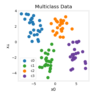
Each dot represents a training example. The axis (x0,x1) are the inputs and the color represents the class the example is associated with. Once trained, the model will be presented with a new example, (x0,x1), and will predict the class.
While generated, this data set is representative of many real-world classification problems. There are several input features (x0,…,xn) and several output categories. The model is trained to use the input features to predict the correct output category.
# show classes in data set
print(f"unique classes {np.unique(y_train)}")
# show how classes are represented
print(f"class representation {y_train[:10]}")
# show shapes of our dataset
print(f"shape of X_train: {X_train.shape}, shape of y_train: {y_train.shape}")
Output
unique classes [0 1 2 3]
class representation [3 3 3 0 3 3 3 3 2 0]
shape of X_train: (100, 2), shape of y_train: (100,)
2.2 Model

This lab will use a 2-layer network as shown.
Unlike the binary classification networks, this network has four outputs, one for each class. Given an input example, the output with the highest value is the predicted class of the input.
Below is an example of how to construct this network in Tensorflow. Notice the output layer uses a linear rather than a softmax activation. While it is possible to include the softmax in the output layer, it is more numerically stable if linear outputs are passed to the loss function during training. If the model is used to predict probabilities, the softmax can be applied at that point.
tf.random.set_seed(1234)  # applied to achieve consistent results
model = Sequential([Dense(2, activation = 'relu',   name = "L1"),Dense(4, activation = 'linear', name = "L2")]
)
The statements below compile and train the network. Setting from_logits=True as an argument to the loss function specifies that the output activation was linear rather than a softmax.
model.compile(loss=tf.keras.losses.SparseCategoricalCrossentropy(from_logits=True),optimizer=tf.keras.optimizers.Adam(0.01),
)model.fit(X_train,y_train,epochs=200
)
With the model trained, we can see how the model has classified the training data.
plt_cat_mc(X_train, y_train, model, classes)
Output
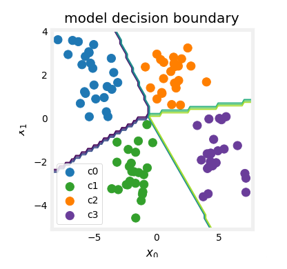
Above, the decision boundaries show how the model has partitioned the input space. This very simple model has had no trouble classifying the training data. How did it accomplish this? Let’s look at the network in more detail.
Below, we will pull the trained weights from the model and use that to plot the function of each of the network units. Further down, there is a more detailed explanation of the results. You don’t need to know these details to successfully use neural networks, but it may be helpful to gain more intuition about how the layers combine to solve a classification problem.
# gather the trained parameters from the first layer
l1 = model.get_layer("L1")
W1,b1 = l1.get_weights()
# plot the function of the first layer
plt_layer_relu(X_train, y_train.reshape(-1,), W1, b1, classes)
Output
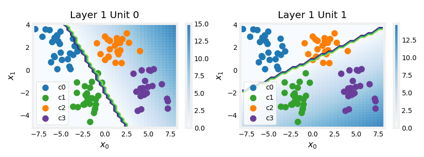
# gather the trained parameters from the output layer
l2 = model.get_layer("L2")
W2, b2 = l2.get_weights()
# create the 'new features', the training examples after L1 transformation
Xl2 = np.maximum(0, np.dot(X_train,W1) + b1)plt_output_layer_linear(Xl2, y_train.reshape(-1,), W2, b2, classes,x0_rng = (-0.25,np.amax(Xl2[:,0])), x1_rng = (-0.25,np.amax(Xl2[:,1])))
Output
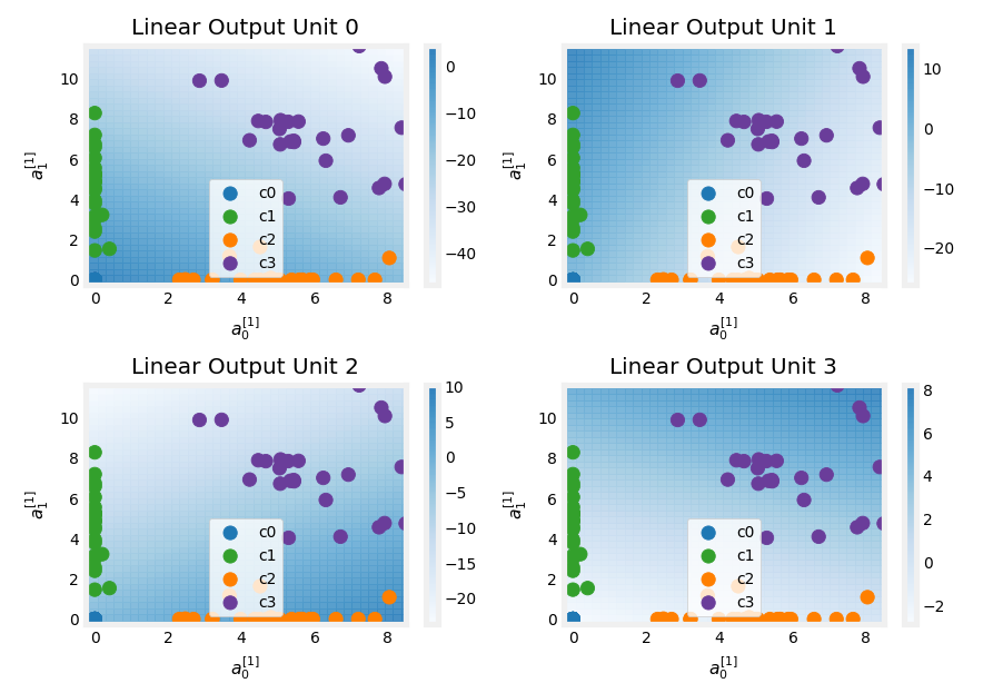
Explanation
Layer 1
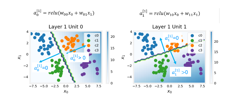
These plots show the function of Units 0 and 1 in the first layer of the network. The inputs are ( x 0 , x 1 x_0,x_1 x0,x1) on the axis. The output of the unit is represented by the color of the background. This is indicated by the color bar on the right of each graph. Notice that since these units are using a ReLu, the outputs do not necessarily fall between 0 and 1 and in this case are greater than 20 at their peaks.
The contour lines in this graph show the transition point between the output, a j [ 1 ] a^{[1]}_j aj[1] being zero and non-zero. Recall the graph for a ReLu :
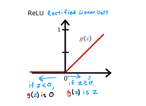
The contour line in the graph is the inflection point in the ReLu.
Unit 0 has separated classes 0 and 1 from classes 2 and 3. Points to the left of the line (classes 0 and 1) will output zero, while points to the right will output a value greater than zero.
Unit 1 has separated classes 0 and 2 from classes 1 and 3. Points above the line (classes 0 and 2 ) will output a zero, while points below will output a value greater than zero. Let’s see how this works out in the next layer!
Layer 2, the output layer
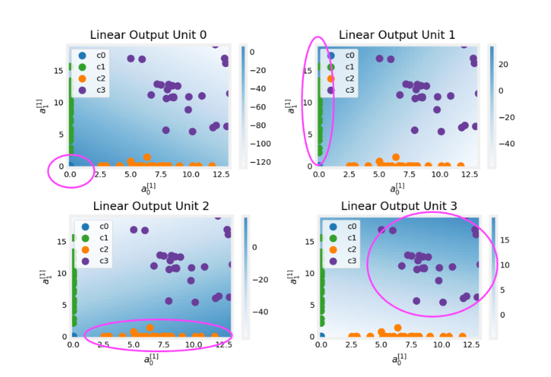
The dots in these graphs are the training examples translated by the first layer. One way to think of this is the first layer has created a new set of features for evaluation by the 2nd layer. The axes in these plots are the outputs of the previous layer a 0 [ 1 ] a^{[1]}_0 a0[1] and a 1 [ 1 ] a^{[1]}_1 a1[1]. As predicted above, classes 0 and 1 (blue and green) have a 0 [ 1 ] = 0 a^{[1]}_0 = 0 a0[1]=0 while classes 0 and 2 (blue and orange) have a 1 [ 1 ] = 0 a^{[1]}_1 = 0 a1[1]=0.
Once again, the intensity of the background color indicates the highest values.
Unit 0 will produce its maximum value for values near (0,0), where class 0 (blue) has been mapped.
Unit 1 produces its highest values in the upper left corner selecting class 1 (green).
Unit 2 targets the lower right corner where class 2 (orange) resides.
Unit 3 produces its highest values in the upper right selecting our final class (purple).
One other aspect that is not obvious from the graphs is that the values have been coordinated between the units. It is not sufficient for a unit to produce a maximum value for the class it is selecting for, it must also be the highest value of all the units for points in that class. This is done by the implied softmax function that is part of the loss function (SparseCategoricalCrossEntropy). Unlike other activation functions, the softmax works across all the outputs.
You can successfully use neural networks without knowing the details of what each unit is up to. Hopefully, this example has provided some intuition about what is happening under the hood.
[6] Practice quiz: Multiclass Classification
Practice quiz: Multiclass Classification
Latest Submission Grade 100%
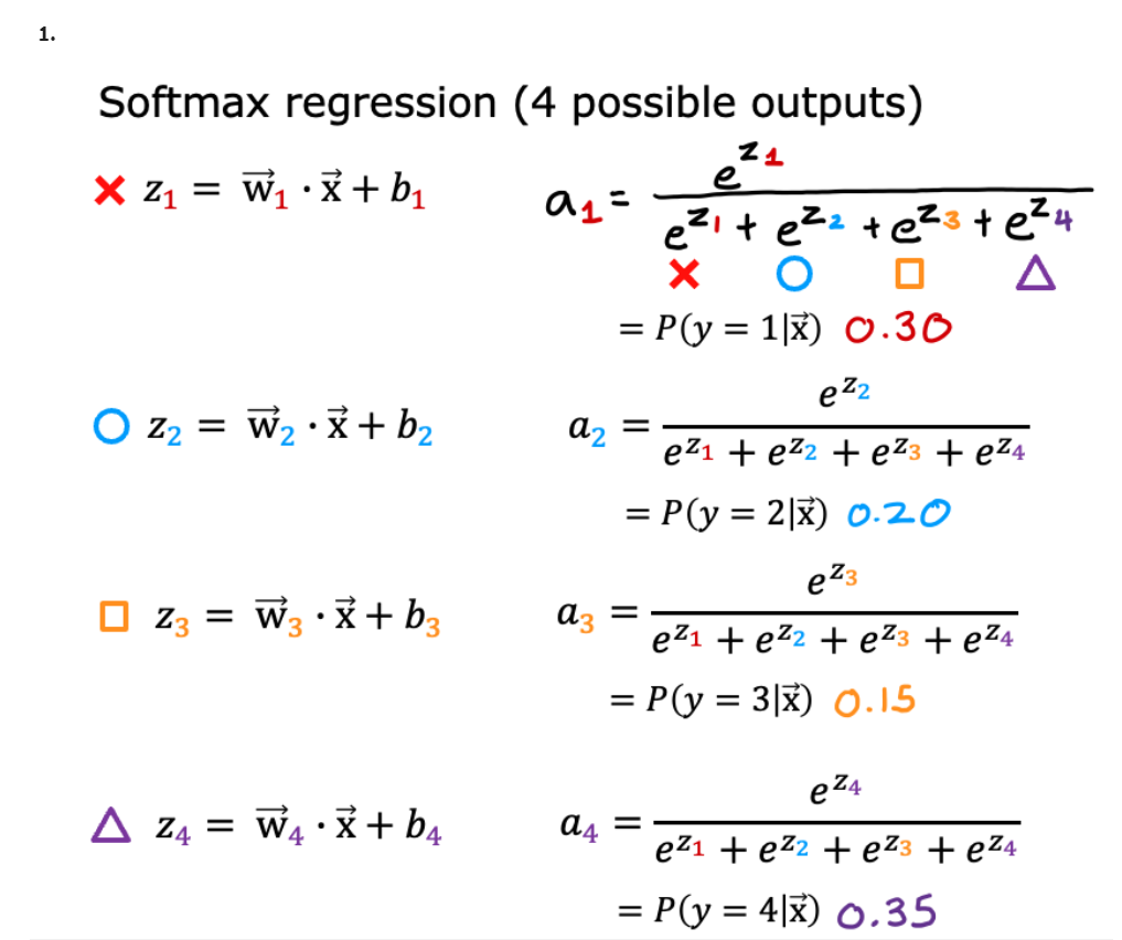
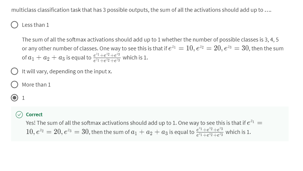

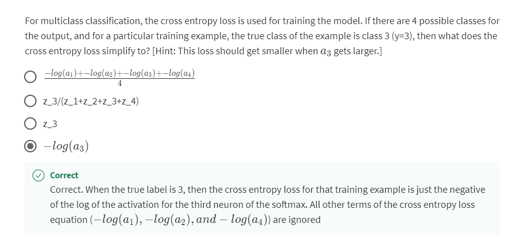
Correct. When the true label is 3, then the cross entropy loss for that training example is just the negative of the log of the activation for the third neuron of the softmax. All other terms of the cross entropy loss equation ( − l o g ( a 1 ) , − l o g ( a 2 ) , a n d − l o g ( a 4 ) -log(a_1),-log(a_2), and -log(a_4) −log(a1),−log(a2),and−log(a4)) are ignored
Question 3
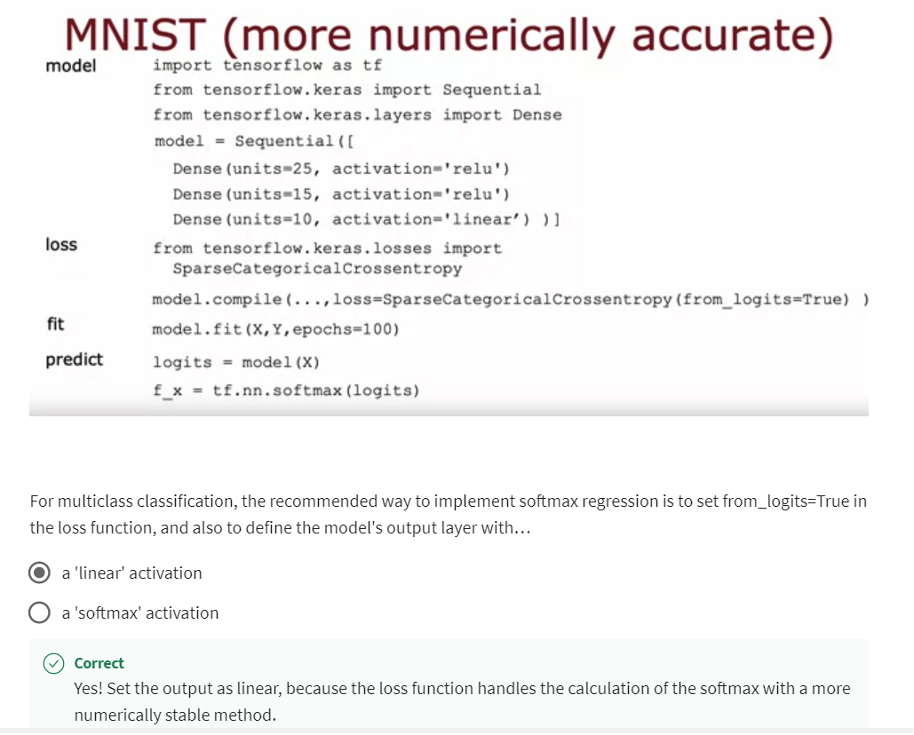
[7] Additional Neural Network Concepts
Advanced Optimization
Gradient descent is an
optimization algorithm that is widely used
in machine learning, and was the foundation
of many algorithms like linear regression and
logistic regression and early implementations
of neural networks.
There are some other optimization algorithms for minimizing the cost function, that are even better than gradient descent.
But it turns out
that there are now some other optimization
algorithms for minimizing the
cost function, that are even better
than gradient descent.
In this video, we’ll take a look at an algorithm
that can help you train your neural network much faster than
gradient descent.
Recall that this is the expression for one
step of gradient descent.A parameter w_j
is updated as w_j minus the learning
rate Alpha times this partial derivative term.How can we make this
work even better?
Minimum of cost function is at the center of ellipsis
In this example, I’ve
plotted the cost function J using a contour plot
comprising these ellipsis, and the minimum of
this cost function is at the center of this
ellipsis down here.

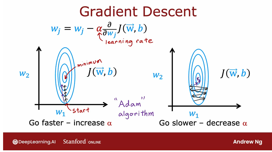
Adam: Adaptive Moment estimation
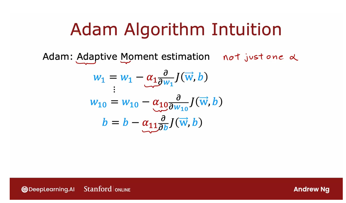
Adam
| Parameters keep moving in same direction | Parameters keep oscillating |
|---|---|
| Increase learning rate alpha | Decrease learning rate alpha |
Now, if you were to start
gradient descent down here, one step of gradient descent, if Alpha is small, may take you a little
bit in that direction.Then another step,
then another step, then another step,
then another step, and you notice that
every single step of gradient descent is pretty much going in the same direction, and if you see this
to be the case, you might wonder, well, why don’t we make Alpha bigger, can we have an algorithm to
automatically increase Alpha?
Adam algorithm
They just make it
take bigger steps and get to the minimum faster. There’s an algorithm called the Adam algorithm
that can do that.
If it sees that the
learning rate is too small, and we are just taking tiny little steps in a similar
direction over and over, we should just make the
learning rate Alpha bigger.
Oscillating back and forth
In contrast, here again, is the same cost
function if we were starting here and have a relatively big
learning rate Alpha, then maybe one step of gradient
descent takes us here, in the second step
takes us here, third step, and the fourth step, and the fifth step,
and the sixth step, and if you see gradient
descent doing this, is oscillating back and forth.
You can take a more smooth path toward the minimum of the cost function
You’d be tempted to say, well, why don’t we make the
learning rates smaller?The Adam algorithm can also
do that automatically, and with a smaller
learning rate, you can then take
a more smooth path toward the minimum of
the cost function.
The Adam algorithm can adjust the learning rate automatically.
Depending on how gradient
descent is proceeding, sometimes you wish you had a
bigger learning rate Alpha, and sometimes you wish you had a smaller learning rate Alpha. The Adam algorithm can adjust the learning
rate automatically.
Adam stands for Adaptive
Moment Estimation, or A-D-A-M, and don’t worry too much about
what this name means, it’s just what the authors
had called this algorithm.
Adam uses different learning rates for every single parameter of the model
But interestingly,
the Adam algorithm doesn’t use a single global
learning rate Alpha. It uses a different
learning rates for every single
parameter of your model.
If you have parameters w_1
through w_10, as was b, then it actually has 11 learning rate
parameters, Alpha_1, Alpha_2, all the way through
Alpha_10 for w_1 to w_10, as well as I’ll call it
Alpha_11 for the parameter b.The intuition behind
the Adam algorithm is, if a parameter w_j, or b seems to keep on moving in roughly
the same direction.
This is what we saw on the first example on
the previous slide. But if it seems
to keep on moving in roughly the same direction, let’s increase the learning
rate for that parameter. Let’s go faster in
that direction.Conversely, if a parameter keeps oscillating
back and forth, this is what you saw in the second example on
the previous slide. Then let’s not have it keep on oscillating or bouncing
back and forth. Let’s reduce Alpha_j for
that parameter a little bit.
The details of how
Adam does this are a bit complicated and beyond
the scope of this course, but if you take some more advanced deep learning
courses later, you may learn more
about the details of this Adam algorithm, but in codes this is
how you implement it. T
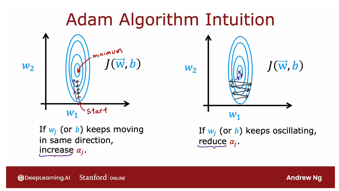
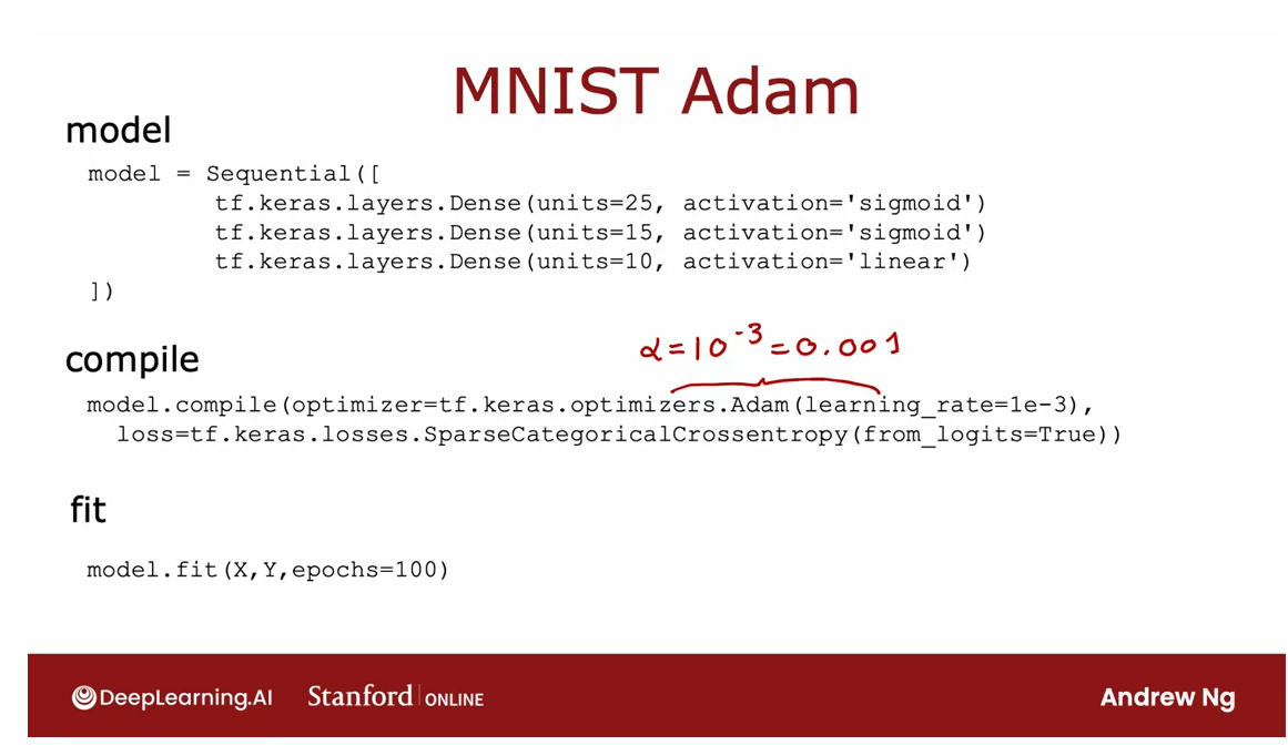
he model is exactly
the same as before, and the way you compile the model is very similar
to what we had before, except that we now add one extra argument to
the compile function, which is that we specify that
the optimizer you want to use is tf.keras.optimizers.Adam
optimizer.
The Adam optimization
algorithm does need some default initial
learning rate Alpha, and in this example, I’ve set that initial learning
rate to be 10^ negative 3.
But when you’re using the
Adam algorithm in practice, it’s worth trying
a few values for this default global
learning rate.Try some large and
some smaller values to see what gives you the
fastest learning performance.
Compared to the original
gradient descent algorithm that you had learned in the
previous course though, the Adam algorithm, because it can adapt
the learning rate a bit automatically, it is more robust to the exact choice of learning
rate that you pick.Though there’s still way tuning this parameter little bit to see if you can get somewhat
faster learning. That’s it for the Adam
optimization algorithm.
It typically works much
faster than gradient descent, and it’s become a
de facto standard in how practitioners train
their neural networks.
If you’re trying to decide what learning algorithm to use, what optimization algorithm to use to train your
neural network. A safe choice would be to just use the Adam
optimization algorithm, and most practitioners
today will use Adam rather than the optional
gradient descent algorithm, and with this, I hope that your learning algorithms will be able to learn much more quickly.
Now, in the next
couple of videos, I’d like to touch on some more advanced concepts
for neural networks, and in particular,
in the next video, let’s take a look at some
alternative layer types.
Additional Layer Types
Dense layer: every neuron in the layer gets its inputs all the activations from the previous layer.
All the neural network layers with you so far have been the dense layer type in
which every neuron in the layer gets its inputs all the activations
from the previous layer.And it turns out that just
using the dense layer type, you can actually build some pretty
powerful learning algorithms. And to help you build further intuition
about what neural networks can do.
It turns out that there’s some other types
of layers as well with other properties. In this video I’d like to
briefly touch on this and give you an example of a different
type of neural network layer.
Let’s take a look to recap in
the dense layer that we’ve been using the activation of a neuron
in say the second hidden layer Is a function of every single activation
value from the previous layer of a one.But it turns out that for
some applications, someone designing a neural network may
choose to use a different type of layer.

Convolutional Layer
One other layer type that you may see in
some work is called a convolutional layer. Let me illustrate this with an example.
So what I’m showing on
the left is the input X. Which is a handwritten digit nine. And what I’m going to do is
construct a hidden layer which will compute different activations
as functions of this input image X.
But here’s something I can do for
the first hidden unit, which I’ve drawn in blue rather than saying this neuron can
look at all the pixels in this image.I might say this neuron can only
look at the pixels in this little rectangular region.
Second neuron, which I’m going to
illustrate in magenta is also not going to look at the entire
input image X instead, it’s only going to look at the pixels
in a limited region of the image.And so on for the third neuron and
the 4th neuron and so on and so forth. Down to the last neuron which may be
looking only at that region of the image.
So why might you want to do this? Why won’t you let every neuron
look at all the pixels but instead look at only some of the pixels?
Look at only part of the input
Well, some of the benefits are first,
it speeds up computation.And second advantage is that a neural
network that uses this type of layer called a convolutional layer
can need less training data or alternatively, it can also be
less prone to overfitting.
You heard me talk a bit about
overfitting in their previous course but this is something that will dive into
greater detail on next week as well.
Convolution layer: Each neuron only looks at a region of the input image
When we talk about practical tips for
using learning algorithms and this is the type of layer where
each neuron only looks at a region of the input image is
called a convolutional layer.
It was a researcher John Macoun who
had figured out a lot of the details of how to get convolutional layers
to work and popularized their use.

Convolutional Neural Network
Let me illustrate in more
detail a convolutional layer.And if you have multiple convolutional
layers in a neural network sometimes that’s called
a convolutional neural network.
To illustrate the convolutional
layer of convolutional neural network on this slide I’m going to
use instead of a two D image input.
Example: electrocardiogram
I’m going to use a one dimensional
input and the motivating example I’m going to use is classification of
E K G signals or electrocardiograms.
So if you put two electrodes on your chest
you will record the voltages that look like this that correspond
to your heartbeat.This is actually something that my
stanford research group did research on.
We were actually reading E K G signals
that actually look like this to try to diagnose if patients
may have a heart issue.So an E K G signal and electoral cardia
graham E C G in some places E K G. In some places there’s just
a list of numbers corresponding to the height of the surface
at different points in time.
So you may have say 100 numbers
corresponding to the height of this curve at 100 different points of time. And the learning tosses
given this time series, given this E K G signal to
classify say whether this patient has a heart disease or
some diagnosable heart conditions.
Here’s what the convolutional
neural network might do. So I’m going to take the E K G signal and
rotated 90 degrees to lay it on the side.And so we have here 100 inputs X one
X two all the way through X 100. Like.So and when I construct the first hidden layer Instead of having the first hidden
unit take us input all 100 numbers.
Let me have the first hidden unit. Look at only X one through X 20. So that corresponds to looking at just
a small window of this E K G signal.
The second hidden layer shown
in a different color here. Well look at X 11 through X 30, so looks at a different window
in this E K G signal.And the third hidden there looks at
another window X21 through X 40 and so on.And the final hidden
units in this example. Well Look at X 81 through X100. So it looks like a small window towards
the end of this EKG time series.So this is a convolutional layer because
these units in this layer looks at only a limited window of the input.
Now this layer of the neural
network has nine units. The next layer can also
be a convolutional layer.
So in the second hidden layer let
me architect my first unit not to look at all nine activations
from the previous layer, but to look at say just the first 5
activations from the previous layer.
And then my second unit In
this second hidden there may look at just another five numbers,
say A3-A7. And the third and final hidden unit in this layer
will only look at A5 through A9.And then maybe finally these activations. A2 gets inputs to a sigmoid unit
that does look at all three of these values of A2 in order to
make a binary classification regarding the presence or
absence of heart disease.
So this is the example of a neural
network with the first hidden layer being a convolutional layer.The second hidden layer also
being a convolutional layer and then the output layer
being a sigmoid layer.
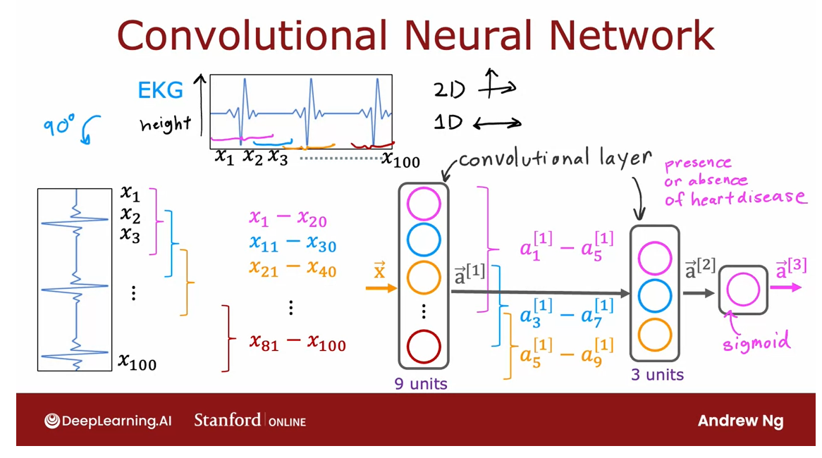
And it turns out that with convolutional
layers you have many architecture choices such as how big is the window of inputs
that a single neuron should look at and how many neurons should layer have.
And by choosing those architectural
parameters effectively, you can build new versions of neural
networks that can be even more effective than the dense layer for
some applications.
To recap, that’s it for the convolutional
layer and convolutional neural networks.I’m not going to go deeper into
convolutional networks in this class and you don’t need to know anything
about them to do the homework and finish this class successfully.
But I hope that you find this
additional intuition that neural networks can have other types
of layers as well to be useful. And in fact, if you sometimes hear
about the latest cutting edge architectures like a transformer model or
an LS TM or an attention model.
A lot of this research in neural networks
even today pertains to researchers trying to invent new types of layers for
neural networks.
And plugging these different types of
layers together as building blocks to form even more complex and
hopefully more powerful neural networks. So that’s it for
the required videos for this week.
Thank you and congrats on sticking
with me all the way through this. And I look forward to seeing you next
week also where we’ll start to talk about practical advice for how you
can build machine learning systems. I hope that the tips you learn next week
will help you become much more effective at building useful
machine learning systems. So I look forward also
to see you next week.
[8] Practice quiz: Additional Neural Network Concepts
Practice quiz: Additional Neural Network Concepts
Latest Submission Grade 100%
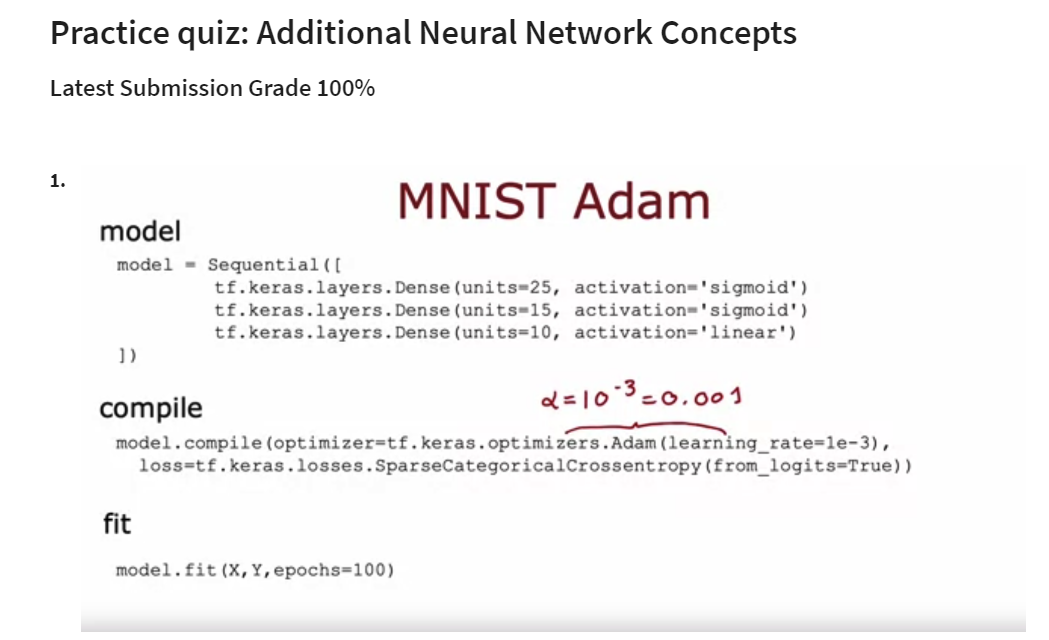
Question 2
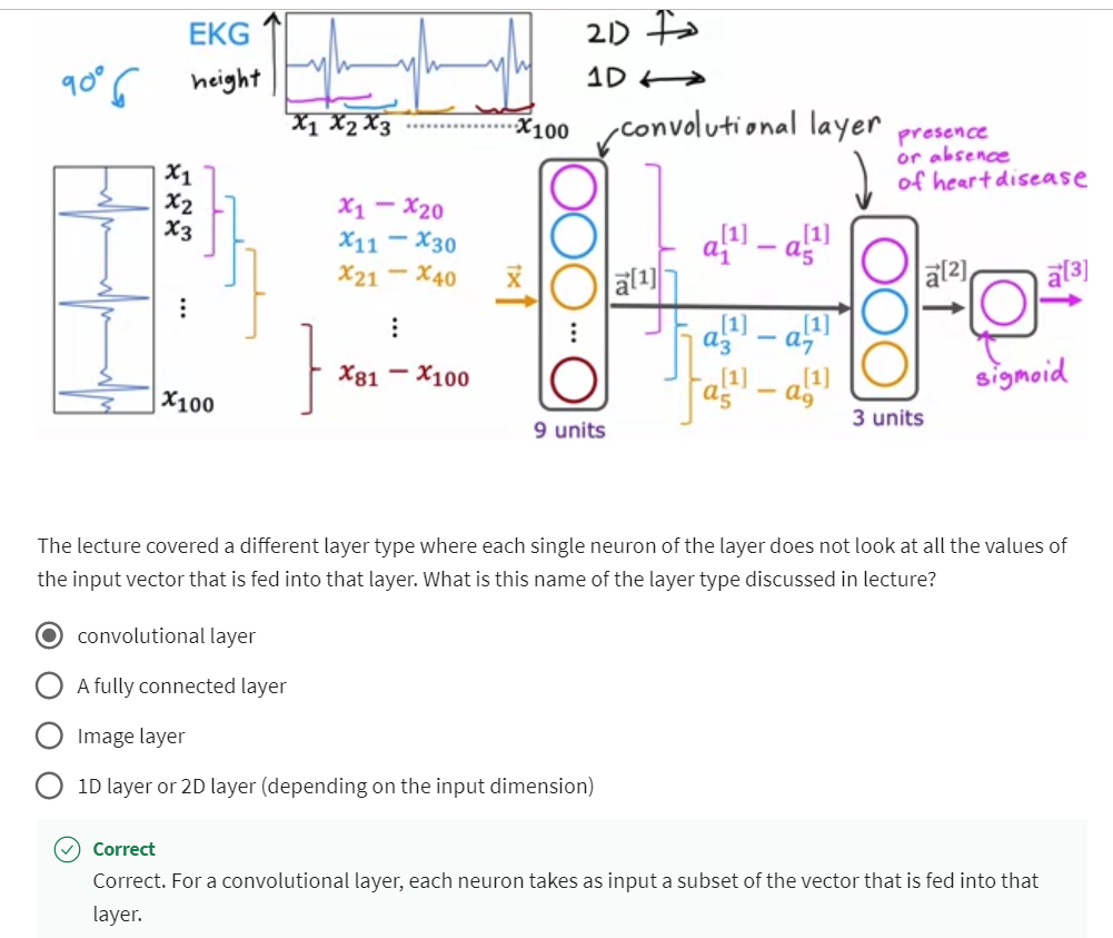
For a convolutional layer, each neuron takes as input a subset of the vector that is fed into that layer.
[9] Practice Lab: Neural network training
Grade Received: 100%

Welcome to this second assignment of course 2. In this exercise, you will extend last weeks assignment to recognize digits 0-9. You will explore the popular ReLu activation as well as the use of the Softmax activation in multiclass classification. You will then build a neural network capable of multiclass classification using the ReLu and Softmax in Tensorflow.
1 - Packages
First, let’s run the cell below to import all the packages that you will need during this assignment.
- numpy is the fundamental package for scientific computing with Python.
- matplotlib is a popular library to plot graphs in Python.
- tensorflow a popular platform for machine learning.
import numpy as np
import tensorflow as tf
from tensorflow.keras.models import Sequential
from tensorflow.keras.layers import Dense
from tensorflow.keras.activations import linear, relu, sigmoid
%matplotlib widget
import matplotlib.pyplot as plt
plt.style.use('./deeplearning.mplstyle')import logging
logging.getLogger("tensorflow").setLevel(logging.ERROR)
tf.autograph.set_verbosity(0)from public_tests import * from autils import *
from lab_utils_softmax import plt_softmax
np.set_printoptions(precision=2)
2 - ReLU Activation
This week, a new activation was introduced, the Rectified Linear Unit (ReLU).
a = m a x ( 0 , z ) ReLU function a = max(0,z) \quad\quad\text { ReLU function} a=max(0,z) ReLU function
plt_act_trio()
Output
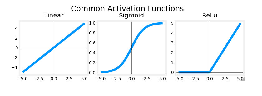
The example from the lecture on the right shows an application of the ReLU. In this example, the derived “awareness” feature is not binary but has a continuous range of values. The sigmoid is best for on/off or binary situations. The ReLU provides a continuous linear relationship. Additionally it has an ‘off’ range where the output is zero.
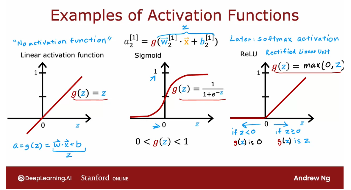
The “off” feature makes the ReLU a Non-Linear activation. Why is this needed? This enables multiple units to contribute to to the resulting function without interfering. This is examined more in the supporting optional lab.
3 - Softmax Function
A multiclass neural network generates N outputs. One output is selected as the predicted answer. In the output layer, a vector z \mathbf{z} z is generated by a linear function which is fed into a softmax function. The softmax function converts z \mathbf{z} z into a probability distribution as described below. After applying softmax, each output will be between 0 and 1 and the outputs will sum to 1. They can be interpreted as probabilities. The larger inputs to the softmax will correspond to larger output probabilities.
最后输出层使用linear层,然后这些结果通过一个额外的Softmax 函数:转化为概率分布
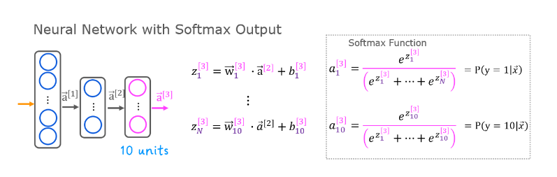
The softmax function can be written:
a j = e z j ∑ k = 0 N − 1 e z k (1) a_j = \frac{e^{z_j}}{ \sum_{k=0}^{N-1}{e^{z_k} }} \tag{1} aj=∑k=0N−1ezkezj(1)
Where z = w ⋅ x + b z = \mathbf{w} \cdot \mathbf{x} + b z=w⋅x+b and N is the number of feature/categories in the output layer.
Exercise 1
Let’s create a NumPy implementation:
这里我使用的是向量版本的代码,性能比较高
# UNQ_C1
# GRADED CELL: my_softmaxdef my_softmax(z):  """ Softmax converts a vector of values to a probability distribution.Args:z (ndarray (N,))  : input data, N featuresReturns:a (ndarray (N,))  : softmax of z"""    ### START CODE HERE ### #a = np.exp(z) / np.sum(np.exp(z)) # my code, passed all the testsez = np.exp(z)a = ez / np.sum(ez)  # reference code, using intermidate variable ez### END CODE HERE ### return a
Test
z = np.array([1., 2., 3., 4.])
a = my_softmax(z)
atf = tf.nn.softmax(z)
print(f"my_softmax(z):         {a}")
print(f"tensorflow softmax(z): {atf}")# BEGIN UNIT TEST
test_my_softmax(my_softmax)
# END UNIT TEST
Output
my_softmax(z):         [0.03 0.09 0.24 0.64]
tensorflow softmax(z): [0.03 0.09 0.24 0.64]All tests passed.
Hint
One implementation uses for loop to first build the denominator and then a second loop to calculate each output.
def my_softmax(z):  N = len(z)a =                     # initialize a to zeros ez_sum =                # initialize sum to zerofor k in range(N):      # loop over number of outputs             ez_sum +=           # sum exp(z[k]) to build the shared denominator      for j in range(N):      # loop over number of outputs again                a[j] =              # divide each the exp of each output by the denominator   return(a)
Hint for code
def my_softmax(z): N = len(z)a = np.zeros(N)ez_sum = 0for k in range(N): ez_sum += np.exp(z[k]) for j in range(N): a[j] = np.exp(z[j])/ez_sum return(a)Or, a vector implementation:def my_softmax(z): ez = np.exp(z) a = ez/np.sum(ez) return(a)
Below, vary the values of the z inputs. Note in particular how the exponential in the numerator magnifies small differences in the values. Note as well that the output values sum to one.
plt.close("all")
plt_softmax(my_softmax)
Output
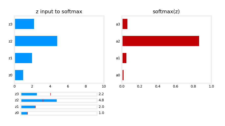
4 - Neural Networks
In last weeks assignment, you implemented a neural network to do binary classification. This week you will extend that to multiclass classification. This will utilize the softmax activation.
4.1 Problem Statement
In this exercise, you will use a neural network to recognize ten handwritten digits, 0-9. This is a multiclass classification task where one of n choices is selected. Automated handwritten digit recognition is widely used today - from recognizing zip codes (postal codes) on mail envelopes to recognizing amounts written on bank checks.
4.2 Dataset
You will start by loading the dataset for this task.
-
The
load_data()function shown below loads the data into variablesXandy -
The data set contains 5000 training examples of handwritten digits 1 ^1 1.
- Each training example is a 20-pixel x 20-pixel grayscale image of the digit.
- Each pixel is represented by a floating-point number indicating the grayscale intensity at that location.
- The 20 by 20 grid of pixels is “unrolled” into a 400-dimensional vector.
- Each training examples becomes a single row in our data matrix
X. - This gives us a 5000 x 400 matrix
Xwhere every row is a training example of a handwritten digit image.
- Each training example is a 20-pixel x 20-pixel grayscale image of the digit.
X = ( − − − ( x ( 1 ) ) − − − − − − ( x ( 2 ) ) − − − ⋮ − − − ( x ( m ) ) − − − ) X = \left(\begin{array}{cc} --- (x^{(1)}) --- \\ --- (x^{(2)}) --- \\ \vdots \\ --- (x^{(m)}) --- \end{array}\right) X= −−−(x(1))−−−−−−(x(2))−−−⋮−−−(x(m))−−−
- The second part of the training set is a 5000 x 1 dimensional vector
ythat contains labels for the training sety = 0if the image is of the digit0,y = 4if the image is of the digit4and so on.
1 ^1 1 This is a subset of the MNIST handwritten digit dataset (http://yann.lecun.com/exdb/mnist/)
# load dataset
X, y = load_data()
4.2.1 View the variables
Let’s get more familiar with your dataset.
- A good place to start is to print out each variable and see what it contains.
The code below prints the first element in the variables X and y.
print ('The first element of X is: ', X[0])
print(X[0].size) # output: 400
Output:
The first element of X is: [ 0.00e+00 0.00e+00 0.00e+00 0.00e+00 0.00e+00 0.00e+00 0.00e+000.00e+00 0.00e+00 0.00e+00 0.00e+00 0.00e+00 0.00e+00 0.00e+000.00e+00 0.00e+00 0.00e+00 0.00e+00 0.00e+00 0.00e+00 0.00e+000.00e+00 0.00e+00 0.00e+00 0.00e+00 0.00e+00 0.00e+00 0.00e+000.00e+00 0.00e+00 0.00e+00 0.00e+00 0.00e+00 0.00e+00 0.00e+000.00e+00 0.00e+00 0.00e+00 0.00e+00 0.00e+00 0.00e+00 0.00e+000.00e+00 0.00e+00 0.00e+00 0.00e+00 0.00e+00 0.00e+00 0.00e+000.00e+00 0.00e+00 0.00e+00 0.00e+00 0.00e+00 0.00e+00 0.00e+000.00e+00 0.00e+00 0.00e+00 0.00e+00 0.00e+00 0.00e+00 0.00e+000.00e+00 0.00e+00 0.00e+00 0.00e+00 8.56e-06 1.94e-06 -7.37e-04-8.13e-03 -1.86e-02 -1.87e-02 -1.88e-02 -1.91e-02 -1.64e-02 -3.78e-03...]
print ('The first element of y is: ', y[0,0])
print ('The last element of y is: ', y[-1,0])
Output
The first element of y is:  0
The last element of y is:  9
4.2.2 Check the dimensions of your variables
Another way to get familiar with your data is to view its dimensions. Please print the shape of X and y and see how many training examples you have in your dataset.
print ('The shape of X is: ' + str(X.shape))
print ('The shape of y is: ' + str(y.shape))
Output
The shape of X is: (5000, 400)
The shape of y is: (5000, 1)
4.2.3 Visualizing the Data
You will begin by visualizing a subset of the training set.
- In the cell below, the code randomly selects 64 rows from
X, maps each row back to a 20 pixel by 20 pixel grayscale image and displays the images together. - The label for each image is displayed above the image
import warnings
warnings.simplefilter(action='ignore', category=FutureWarning)
# You do not need to modify anything in this cellm, n = X.shapefig, axes = plt.subplots(8,8, figsize=(5,5))
fig.tight_layout(pad=0.13,rect=[0, 0.03, 1, 0.91]) #[left, bottom, right, top]#fig.tight_layout(pad=0.5)
widgvis(fig)
for i,ax in enumerate(axes.flat):# Select random indicesrandom_index = np.random.randint(m)# Select rows corresponding to the random indices and# reshape the imageX_random_reshaped = X[random_index].reshape((20,20)).T# Display the imageax.imshow(X_random_reshaped, cmap='gray')# Display the label above the imageax.set_title(y[random_index,0])ax.set_axis_off()fig.suptitle("Label, image", fontsize=14)
Output
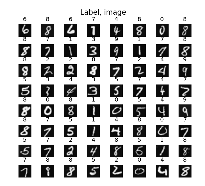
4.3 Model representation
The neural network you will use in this assignment is shown in the figure below.
- This has two dense layers with ReLU activations followed by an output layer with a linear activation.
- Recall that our inputs are pixel values of digit images.
- Since the images are of size 20 × 20 20\times20 20×20, this gives us 400 400 400 inputs
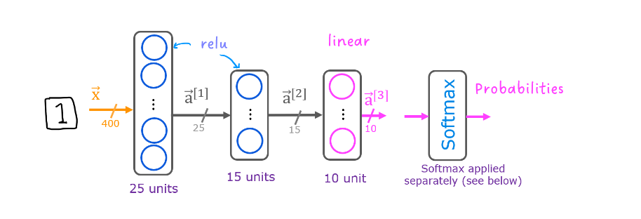
-
The parameters have dimensions that are sized for a neural network with 25 25 25 units in layer 1, 15 15 15 units in layer 2 and 10 10 10 output units in layer 3, one for each digit.
-
Recall that the dimensions of these parameters is determined as follows:
- If network has s i n s_{in} sin units in a layer and s o u t s_{out} sout units in the next layer, then
- W W W will be of dimension s i n × s o u t s_{in} \times s_{out} sin×sout.
- b b b will be a vector with s o u t s_{out} sout elements
- If network has s i n s_{in} sin units in a layer and s o u t s_{out} sout units in the next layer, then
-
Therefore, the shapes of
W, andb, are- layer1: The shape of
W1is (400, 25) and the shape ofb1is (25,) - layer2: The shape of
W2is (25, 15) and the shape ofb2is: (15,) - layer3: The shape of
W3is (15, 10) and the shape ofb3is: (10,)
- layer1: The shape of
-
Note: The bias vector
bcould be represented as a 1-D (n,) or 2-D (n,1) array. Tensorflow utilizes a 1-D representation and this lab will maintain that convention:
4.4 Tensorflow Model Implementation
Tensorflow models are built layer by layer. A layer’s input dimensions ( s i n s_{in} sin above) are calculated for you. You specify a layer’s output dimensions and this determines the next layer’s input dimension. The input dimension of the first layer is derived from the size of the input data specified in the model.fit statement below.
Note: It is also possible to add an input layer that specifies the input dimension of the first layer. For example:
tf.keras.Input(shape=(400,)), #specify input shape
We will include that here to illuminate some model sizing.
4.5 Softmax placement
As described in the lecture and the optional softmax lab, numerical stability is improved if the softmax is grouped with the loss function rather than the output layer during training. This has implications when building the model and using the model.
Building:
- The final Dense layer should use a ‘linear’ activation. This is effectively no activation.
- The
model.compilestatement will indicate this by includingfrom_logits=True.
loss=tf.keras.losses.SparseCategoricalCrossentropy(from_logits=True) - This does not impact the form of the target. In the case of SparseCategorialCrossentropy, the target is the expected digit, 0-9.
Using the model:
- The outputs are not probabilities. If output probabilities are desired, apply a softmax function.
Expected Output
The `model.summary()` function displays a useful summary of the model. Note, the names of the layers may vary as they are auto-generated unless the name is specified.
Model: "my_model"
_________________________________________________________________
Layer (type)                 Output Shape              Param #
=================================================================
L1 (Dense)                   (None, 25)                10025
_________________________________________________________________
L2 (Dense)                   (None, 15)                390
_________________________________________________________________
L3 (Dense)                   (None, 10)                160
=================================================================
Total params: 10,575
Trainable params: 10,575
Non-trainable params: 0
_________________________________________________________________
Exercise 2
Below, using Keras Sequential model and Dense Layer with a ReLU activation to construct the three layer network described above.
这里需要自己写Input的维度,另外每个Dense层添加名字
# UNQ_C2
# GRADED CELL: Sequential model
tf.random.set_seed(1234) # for consistent results
model = Sequential([               ### START CODE HERE ### tf.keras.Input(shape=(400,)),Dense(units=25, activation="relu", name="L1"),Dense(units=15, activation="relu", name="L2"),Dense(units=10, activation="linear", name="L3")### END CODE HERE ### ], name = "my_model"
)
Use summary to take a look at the structure
model.summary()
Output
Model: "my_model"
_________________________________________________________________Layer (type)                Output Shape              Param #
=================================================================L1 (Dense)                  (None, 25)                10025     L2 (Dense)                  (None, 15)                390       L3 (Dense)                  (None, 10)                160       =================================================================
Total params: 10,575
Trainable params: 10,575
Non-trainable params: 0
_________________________________________________________________
Hints
tf.random.set_seed(1234)
model = Sequential([               ### START CODE HERE ### tf.keras.Input(shape=(400,)),     # @REPLACE Dense(25, activation='relu', name = "L1"), # @REPLACE Dense(15, activation='relu',  name = "L2"), # @REPLACE  Dense(10, activation='linear', name = "L3"),  # @REPLACE ### END CODE HERE ### ], name = "my_model"
)
Unit test
# BEGIN UNIT TEST
test_model(model, 10, 400)
# END UNIT TEST
Output
All tests passed!
The parameter counts shown in the summary correspond to the number of elements in the weight and bias arrays as shown below.
Let’s further examine the weights to verify that tensorflow produced the same dimensions as we calculated above.
[layer1, layer2, layer3] = model.layers#### Examine Weights shapes
W1,b1 = layer1.get_weights()
W2,b2 = layer2.get_weights()
W3,b3 = layer3.get_weights()
print(f"W1 shape = {W1.shape}, b1 shape = {b1.shape}")
print(f"W2 shape = {W2.shape}, b2 shape = {b2.shape}")
print(f"W3 shape = {W3.shape}, b3 shape = {b3.shape}")
Output
W1 shape = (400, 25), b1 shape = (25,)
W2 shape = (25, 15), b2 shape = (15,)
W3 shape = (15, 10), b3 shape = (10,)
Expected Output
W1 shape = (400, 25), b1 shape = (25,)
W2 shape = (25, 15), b2 shape = (15,)
W3 shape = (15, 1), b3 shape = (10,)
The following code:
- defines a loss function,
SparseCategoricalCrossentropyand indicates the softmax should be included with the loss calculation by addingfrom_logits=True) - defines an optimizer. A popular choice is Adaptive Moment (Adam) which was described in lecture.
model.compile(loss=tf.keras.losses.SparseCategoricalCrossentropy(from_logits=True),optimizer=tf.keras.optimizers.Adam(learning_rate=0.001),
)history = model.fit(X,y,epochs=40
)
Epochs and batches
In the compile statement above, the number of epochs was set to 100. This specifies that the entire data set should be applied during training 100 times. During training, you see output describing the progress of training that looks like this:
Epoch 1/100
157/157 [==============================] - 0s 1ms/step - loss: 2.2770
The first line, Epoch 1/100, describes which epoch the model is currently running. For efficiency, the training data set is broken into ‘batches’. The default size of a batch in Tensorflow is 32. There are 5000 examples in our data set or roughly 157 batches. The notation on the 2nd line 157/157 [==== is describing which batch has been executed.
Loss (cost)
In course 1, we learned to track the progress of gradient descent by monitoring the cost. Ideally, the cost will decrease as the number of iterations of the algorithm increases. Tensorflow refers to the cost as loss. Above, you saw the loss displayed each epoch as model.fit was executing. The .fit method returns a variety of metrics including the loss. This is captured in the history variable above. This can be used to examine the loss in a plot as shown below.
plot_loss_tf(history)
Output
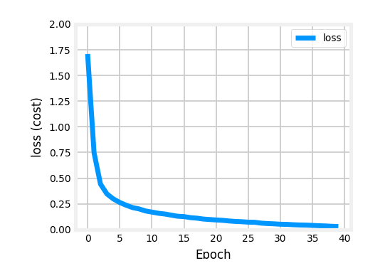
Prediction
To make a prediction, use Keras predict. Below, X[1015] contains an image of a two.
image_of_two = X[1015]
display_digit(image_of_two)prediction = model.predict(image_of_two.reshape(1,400))  # predictionprint(f" predicting a Two: \n{prediction}")
print(f" Largest Prediction index: {np.argmax(prediction)}")
Output
Ignore an image of digit 2 here
 predicting a Two:
[[ -7.99  -2.23   0.77  -2.41 -11.66 -11.15  -9.53  -3.36  -4.42  -7.17]]Largest Prediction index: 2
The largest output is prediction[2], indicating the predicted digit is a ‘2’. If the problem only requires a selection, that is sufficient. Use NumPy argmax to select it. If the problem requires a probability, a softmax is required:
prediction_p = tf.nn.softmax(prediction)print(f" predicting a Two. Probability vector: \n{prediction_p}")
print(f"Total of predictions: {np.sum(prediction_p):0.3f}")
Output
 predicting a Two. Probability vector:
[[1.42e-04 4.49e-02 8.98e-01 3.76e-02 3.61e-06 5.97e-06 3.03e-05 1.44e-025.03e-03 3.22e-04]]
Total of predictions: 1.000
To return an integer representing the predicted target, you want the index of the largest probability. This is accomplished with the Numpy argmax function.
yhat = np.argmax(prediction_p)print(f"np.argmax(prediction_p): {yhat}")
Output
np.argmax(prediction_p): 2
Let’s compare the predictions vs the labels for a random sample of 64 digits. This takes a moment to run.
import warnings
warnings.simplefilter(action='ignore', category=FutureWarning)
# You do not need to modify anything in this cellm, n = X.shapefig, axes = plt.subplots(8,8, figsize=(5,5))
fig.tight_layout(pad=0.13,rect=[0, 0.03, 1, 0.91]) #[left, bottom, right, top]
widgvis(fig)
for i,ax in enumerate(axes.flat):# Select random indicesrandom_index = np.random.randint(m)# Select rows corresponding to the random indices and# reshape the imageX_random_reshaped = X[random_index].reshape((20,20)).T# Display the imageax.imshow(X_random_reshaped, cmap='gray')# Predict using the Neural Networkprediction = model.predict(X[random_index].reshape(1,400))prediction_p = tf.nn.softmax(prediction)yhat = np.argmax(prediction_p)# Display the label above the imageax.set_title(f"{y[random_index,0]},{yhat}",fontsize=10)ax.set_axis_off()
fig.suptitle("Label, yhat", fontsize=14)
plt.show()
Output
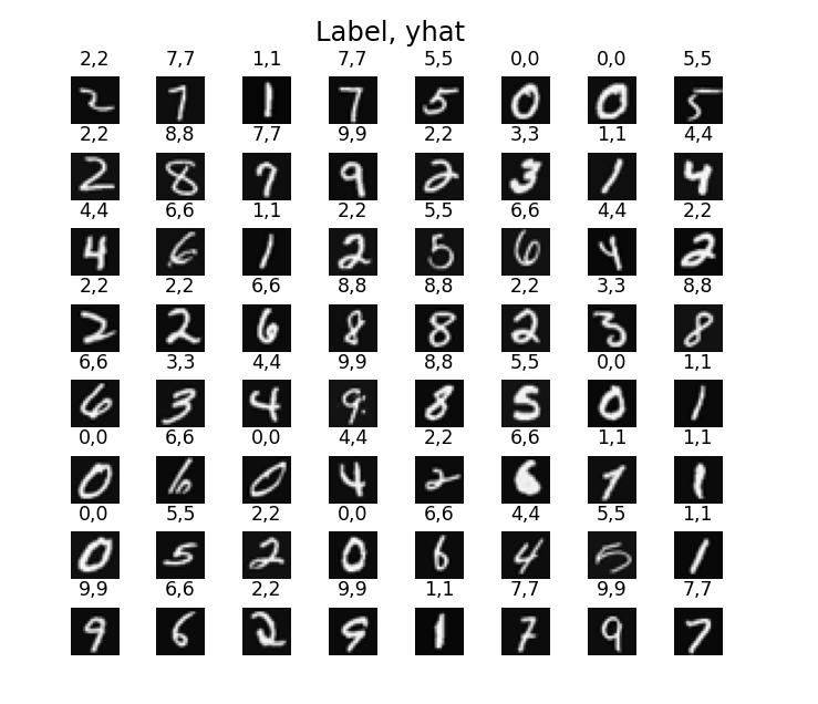
Let’s look at some of the errors.
Note: increasing the number of training epochs can eliminate the errors on this data set.
print( f"{display_errors(model,X,y)} errors out of {len(X)} images")
Output
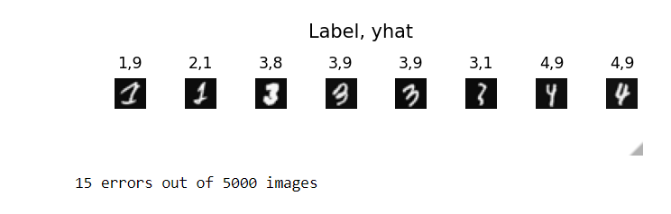
Congratulations!
You have successfully built and utilized a neural network to do multiclass classification.
其他
commit
git commit -m "Finish xxx part of week xx of Advanced Learning Algorithms"
For example
git commit -m "Finish '[7] Additional Neural Network Concepts' and '[8] Practice quiz: Additional Neural Network Concepts' part of week 02 of Advanced Learning Algorithms"
Without formatting
git commit -m "Finish Practice quiz: Neural network model part of week 02 of Advanced Learning Algorithms, without formating the transcript"
Reformat transcript
git commit -m "Reformat learning notes of Example: Recognizing Images part of week 01 of Advanced Learning Algorithms"
practice lab folder name
week02_work_advance_learning_algorithm
2022年6月25日17点17分我的 Cousera 课程学习情况

Course name:
Advanced Learning Algorithms
英文发音
numerator:分子
electrocardiograms
美 [ɪˌlektroʊˈkɑːrdioʊɡræm]
记忆技巧:electro 电 + cardio〔= cardi〕心,心脏 + gram 写,画 → 画心脏跳动的电路图 → 心电图
I’d like to touch on some more advanced concepts for neural networks:接触一些高级概念
oscillating 英 [ˈɒsɪleɪtɪŋ] 摇摆,变化,来回摆动,振荡
legible:英 [ˈledʒəbl] ,清晰的,易读的
One downside of this code is it becomes a little bit less legible. 此代码的一个缺点是它变得不太清晰。
That works okay
Numerical round-off errors aren’t that bad.
For logistic regression, this works okay, and usually the numerical round-off errors aren’t that bad.
Let’s take a look at what can go wrong with that implementation and also how to make it better.
看一下这种方式有什么问题
this name is a bit of a mouthful: 这个名字有点拗口
mouthful: 名词,a mouthful 又长又拗口的词
embellish:修饰
carry out multiclass classification problems: 实施多分类问题
a pharmaceutical company
pharmaceutical 制药的,英 [ˌfɑːməˈsuːtɪkl]
do a quick web search: 搜索
that’s done with this code snippet: 这段代码就是解决这个的
arcane: 神秘的,难懂的
rewind this video:重放此视频
not counting the input layer: 不计算(计数)输入层
subroutine: 子程序
向量转置:taking the first column of A and laying it on the side like this: 把这一列变成一行
string together: 串起来
underscore : 下划线
double square bracket: [[ ]]
coffee roasting: 咖啡烘焙
is getting a little bit cluttered: 变得杂乱无章
方括号:square bracket, []
superscript in square brackets 1: 上标是方括号1,[1]
carry out this task: 做这个任务
Biological neuron:
nucleus of the neuron: 神经元核
dendrites: 树突 ˈdendrīt
axon:轴突 ˈakˌsän
make inroads into 有巨大的影响力;取得进步
they gained in popularity again:火了
it fell out of favor for a while: 失宠了一段时间