1. 概念
1.1. MTBF
MTBF(Mean Time Between Failure),平均故障间隔时间,也被称为平均无故障时间,是衡量一个产品的可靠性指标,其单位为小时。其定义为:产品在总的使用阶段累计工作时间与故障次数的比值:
MTBF用于衡量可修复故障的产品,其统计所有样本的因为故障停机到开机之间的时间间隔和,再除以总故障数,即为平均无故障时间。(MTBF不包括故障发现后的停机和维修时间)
1.2. 故障率
故障率λ是指在单位时间内产品出现故障的概率,通常以每百万小时为单位进行统计。每百万小时一个故障称为一个FIT(Failures in time)。MTBF=1/λ,1FIT时对应的MTBF为1/1FIT=100万小时。所以求解MTBF也可以通过求解故障率来进行。
1.3. 阿伦尼乌斯公式
阿伦尼乌斯公式(Arrhenius equation )是化学术语,是瑞典的阿伦尼乌斯所创立的化学反应速率常数随温度变化关系的经验公式。其公式指数形式:k=Ae^{-Ea/RT} (k为速率常数,R为摩尔气体常量,T为热力学温度,Ea为表观活化能,A为前因子也称为阿伦尼乌斯常数, e为自然对数的底)。
1.4. 半导体老化加速因子
为了测试产品故障率,正常情况下可能需要几年甚至十几年,这个时间太长了,无法实践。为了加强测试产品故障率,会引入一些老化加速条件。JEDEC协会依据阿伦尼乌斯公式,通过提升温度,可以加速产品老化。通过经验,JEDEC将阿伦尼乌斯公式中的A定为1,那么加速因子AF(Acceleration Factor)公式:
AF=exp[\frac{E_A}{k}\cdot((\frac{1}{T_{use}}-\frac{1}{T_{stress}}))]
玻尔兹曼常数k为1.380649 * 10^{-23} J/K(焦耳/开尔文),可换算为8.617333262145 *10^{-5 e}V/K(电子伏/开尔文), e约等于 2.71828,表观活化能E_A一般情况为0.7eV。
示例:
● 使用温度55ºC,转为绝对温度为273+55=328K。
● 压力温度125ºC,转为绝对温度为273+125=398K。
AF=2.71828^{(\frac{0.7}{0.0000861733}\cdot((\frac{1}{328}-\frac{1}{398})))}=78.6
也就是说在125ºC下测试1小时相当于在55ºC下测试78.6小时。
常见的半导体表观活化能值:
1.5. 双侧置信区间

1.6. 单侧置信区间

1.7. 置信度(置信水平)、置信区间:

置信度,即落到指定置信区域内的概率。
1.8. 卡方分布
若n个相互独立的随机变量ξ₁,ξ₂,…,ξn ,均服从标准正态分布(也称独立同分布于标准正态分布),则这n个服从标准正态分布的随机变量的平方和构成一新的随机变量,其分布规律称为卡方分布(chi-square distribution)。卡方分布是一种常见的概率分布。从图中可以看出,统计的独立变量越多,其分布越趋近于标准的正态分布。
2. 实际测试
实际测试过程中,单片测试存在偶然性,所以会增加测试样品来保证测试数据的准确性。并且为了加速测试,会增加一些加速因子来加速测试流程。故障率的分布是个指数分布,指数函数推导可以得到下面的公式,推导过程见附录3.1。MTTF在大多数情况下和MTBF是近似相等的。
2.1. 单温度加速因子
100个样品,测试400小时,使用125ºC加压测试,只有1个样品在300小时出错,使用60%的置信度下限,90%的置信度上限,那么:
温度加速因子A_i=78.6(参见前文)
2.2. 温度和TBW加速因子
明确提出TWB加速因子的是Micro。假设在典型的使用场景下,一个容量为100GB的固态硬盘(SSD)可以使用5年(43,800小时)。该SSD的寿命指标为175 TBW(总写入数据量)。如果在1008小时内写入了130TB的数据,并且写入放大系数了1.2倍,那么TBW的加速因子为32。如果在短时间内写入更多的数据,TBW的加速因子相应增加。
3. 附录
3.1. 故障率推算过程
For an exponential distribution, the probability density function (pdf) is:

(1)
where λ is the failure rate. In the case of the exponential distribution, the mean time to failure (MTTF) is the inverse of λ:

(2)
Manufacturers are often required to design a test to demonstrate the MTTF or failure rate of a product.
In the DRT tool, there are three methods that can be used for reliability demonstration test design: Parametric Binomial, Non-Parametric Binomial and Exponential Chi-Squared. The first two are based on the binomial distribution. From its name, we also can guess that the third method is based on the Chi-Squared distribution and is designed to be used in cases when the failure time distribution is exponential. The reliability function of an exponential distribution is:

(3)
Because of the one-to-one relationship between the failure rate, MTTF, and reliability at time t, the test plan can be designed based on a requirement for either metric. For example, in Figure 1 the required lower bound of MTTF is 100 at a confidence level of 90%. This is the same as requiring the upper bound of the failure rate to be 1/100 = 0.01, or requiring the lower bound of the reliability at time t to be e-0.01xt.
Defining the accumulated test time as T, the following formula is used for calculating T:

(4)
where r is the number of failures and CL is the confidence level.
The above equation is well-known to many engineers nowadays. However, it was not so well-known 15 years ago according to Gorski [1] who wrote: “Well-known to whom? My guess is that less than 0.1% of reliability and quality assurance engineers know it even though many statisticians do. In my 23 years of industry experience I never met an engineer who knew it and yet I worked on projects such as Minuteman I and Apollo where the intent was to bring on board the best people available.” To popularize its application, Gorski wrote a paper on the formula and showed how to use it to design a test plan by using a Chi-Squared distribution table. These days, it is not a popular idea to use a table and a hand calculator to design a test plan using Eqn. (4).
The question now is: why is Eqn. (4) valid? In other words, why can the Chi-Squared distribution be used for design of reliability demonstration tests? In the following discussion, we will provide an explanation.
When the failure times follow an exponential distribution, the number of failures in the time interval T follows a Poisson distribution with associated parameter λT. The relationship is given by:

where N(T) is the number of events during time T.
The relationship above can then be used to obtain the upper bound of the failure rate λ by solving the following equation:

(5)
where:
● r is the total number of failures.
● CL is the confidence level.
● λ is the failure rate at confidence level of CL.
We can then manipulate Eqn. (5) in a number of steps so that we can show the relationship with the Chi-Squared distribution.
If we define x = λT, then Eqn. (5) becomes:

(6)
Using Eqn. (6), for a given confidence level CL, the corresponding upper bound of the random variable X can be solved for. The upper bound is x, a realization of X. Eqn. (6) in fact shows the cumulative distribution function for the random variable X. It can be rewritten as:

(7)
Eqn. (7) can then be related to the Gamma distribution. For a Gamma distribution Y~Gamma(k,λ), the cumulative distribution function (cdf) is:
(8)
Comparing Eqn. (7) to Eqn. (8), one can see that x follows the Gamma distribution X ~ Gamma(r+1,1). Based on the properties of a Gamma random variable, we know 2X ~ Gamma(r+1,2). In addition, is a special case of the Gamma distribution if the random variable follows Gamma(r+1,2). Therefore, we can also say 2X ~ . Since x = λT, we know the upper bound of the failure rate is:

(9)
From the relationship between the exponential, Gamma and Chi-Squared distributions, we have shown why the Chi-Squared distribution can be used in design of reliability tests when the units to be tested follow an exponential distribution. Two examples of using Eqn. (9) are given next.