线性回归
- 1 一元线性回归重要公式
- 2 一元线性回归code实现
- 3 sklearn实现一元线性回归
- 4 多元线性回归公式
- 5 sklearn实现多元线性回归
- 6 模型评价指标
- 7 多项式回归
- 7.1将多项式回归作为线性回归处理
- 7.2 sklaearn多项式特征维度扩展
1 一元线性回归重要公式
一元线性回归的均方误差:
E ( w , b ) = ∑ i = 1 m ( y i − w x i − b ) 2 {{\rm{E}}_{(w,b)}} = {\sum\limits_{i = 1}^m {({y_i} - w{x_i} - b)} ^2} E(w,b)=i=1∑m(yi−wxi−b)2
对w和b分别求导,得
∂ E ( w , b ) ∂ w = 2 ( w ∑ i = 1 m x i 2 − ∑ i = 1 m ( y i − b ) x i ) \frac{{\partial {E_{(w,b)}}}}{{\partial w}} = 2(w\sum\limits_{i = 1}^m {x_i^2 - \sum\limits_{i = 1}^m {({y_i} - b){x_i}} } ) ∂w∂E(w,b)=2(wi=1∑mxi2−i=1∑m(yi−b)xi)
∂ E ( w , b ) ∂ b = 2 ( m b − ∑ i = 1 m y i − w x i ) \frac{{\partial {E_{(w,b)}}}}{{\partial b}} = 2(mb - \sum\limits_{i = 1}^m {{y_i} - w{x_i}} ) ∂b∂E(w,b)=2(mb−i=1∑myi−wxi)
令以上式子分别等于0,得
w = ∑ i = 1 m y i ( x i − x ˉ ) ∑ i = 1 m x i 2 − 1 m ( ∑ i = 1 m x i ) 2 w = \frac{{\sum\limits_{i = 1}^m {{y_i}({x_i} - \bar x)} }}{{\sum\limits_{i = 1}^m {x_i^2 - \frac{1}{m}{{(\sum\limits_{i = 1}^m {{x_i}} )}^2}} }} w=i=1∑mxi2−m1(i=1∑mxi)2i=1∑myi(xi−xˉ)
b = 1 m ∑ i = 1 m ( y i − w x i ) b = \frac{1}{m}\sum\limits_{i = 1}^m {({y_i} - w{x_i})} b=m1i=1∑m(yi−wxi)
如果用Python 来实现上式的话,上式中的求和运算只能用循环来实现。但是如果能将上式向量化,也就是转换成矩阵(即向量)运算的话,就可以利用诸如NumPy 这种专门加速矩阵运算的类库来进
行编写。
w = ∑ i = 1 m ( x i − x ˉ ) ( y i − y ˉ ) ∑ i = 1 m ( x i − x ˉ ) w = \frac{{\sum\limits_{i = 1}^m {({x_i} - \bar x)({y_i} - \bar y)} }}{{\sum\limits_{i = 1}^m {({x_i} - \bar x)} }} w=i=1∑m(xi−xˉ)i=1∑m(xi−xˉ)(yi−yˉ)
2 一元线性回归code实现
import numpy as np
import pandas as pd
from sklearn import datasets
import matplotlib.pyplot as plt
import warnings
warnings.filterwarnings("ignore")# 该数据集的导入可参考 https://blog.csdn.net/virtualxiaoman/article/details/133844179
# 数据集的具体样式及为什么跳过前22行,参考http://lib.stat.cmu.edu/datasets/boston
# 该数据集各变量描述
'''Variables in order:CRIM per capita crime rate by townZN proportion of residential land zoned for lots over 25,000 sq.ft.INDUS proportion of non-retail business acres per townCHAS Charles River dummy variable (= 1 if tract bounds river; 0 otherwise)NOX nitric oxides concentration (parts per 10 million)RM average number of rooms per dwellingAGE proportion of owner-occupied units built prior to 1940DIS weighted distances to five Boston employment centresRAD index of accessibility to radial highwaysTAX full-value property-tax rate per $10,000PTRATIO pupil-teacher ratio by townB 1000(Bk - 0.63)^2 where Bk is the proportion of blacks by townLSTAT % lower status of the populationMEDV Median value of owner-occupied homes in $1000's
'''
data_url = "http://lib.stat.cmu.edu/datasets/boston"
raw_df = pd.read_csv(data_url, sep="\s+", skiprows=22, header=None)
data = np.hstack([raw_df.values[::2, :], raw_df.values[1::2, :2]])
target = raw_df.values[1::2, 2]
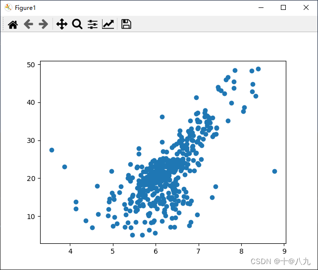
x = data[:, 5]
y = targetx = x[y<50] # 该列数据的最大值是50,不移除的话会存在很多等于50的数据
y = y[y<50]plt.figure(num='Figure1')
plt.scatter(x,y)
plt.show()from sklearn.model_selection import train_test_split
x_train, x_test, y_train, y_test = train_test_split(x, y, test_size = 0.3, random_state = 0)
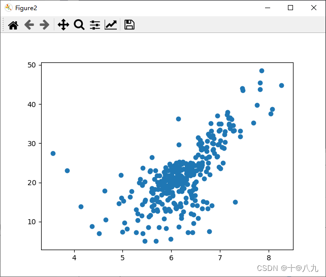
plt.figure(num='Figure2')
plt.scatter(x_train, y_train)
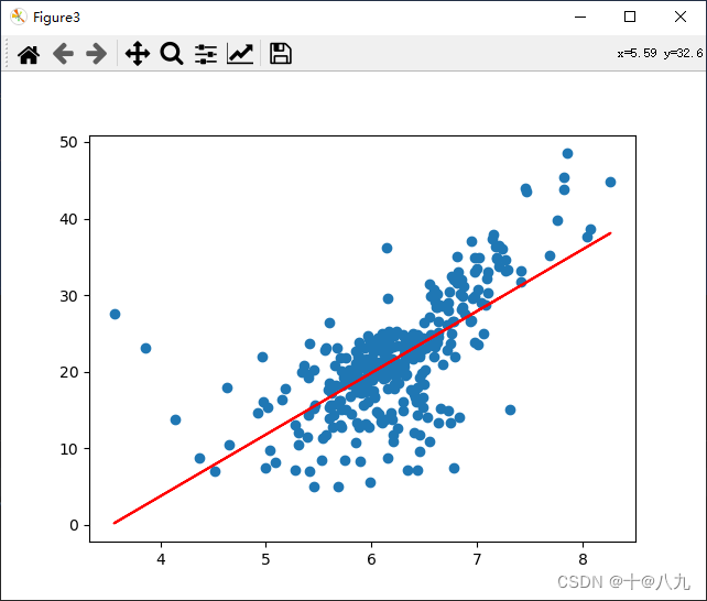
plt.show()def fit(x, y):a_up = np.sum((x-np.mean(x))*(y - np.mean(y)))a_bottom = np.sum((x-np.mean(x))**2)a = a_up / a_bottomb = np.mean(y) - a * np.mean(x)return a, ba, b = fit(x_train, y_train)
plt.figure(num='Figure3')
plt.scatter(x_train, y_train)
plt.plot(x_train, a*x_train+ b, c='r')
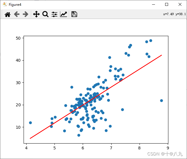
plt.show()plt.figure(num='Figure4')
plt.scatter(x_test, y_test)
plt.plot(x_test, a*x_test+ b, c='r')
plt.show()
3 sklearn实现一元线性回归
import numpy as np
import pandas as pd
from matplotlib import pyplot as plt
from sklearn.model_selection import train_test_split
from sklearn.linear_model import LinearRegressiondata_url = "http://lib.stat.cmu.edu/datasets/boston"
raw_df = pd.read_csv(data_url, sep="\s+", skiprows=22, header=None)
data = np.hstack([raw_df.values[::2, :], raw_df.values[1::2, :2]])
target = raw_df.values[1::2, 2]
x = data[:, 5]
y = target
x = x[y<50] # 该列数据的最大值是50,不移除的话会存在很多等于50的数据
y = y[y<50]lin_reg = LinearRegression()
x_train, x_test, y_train, y_test = train_test_split(x, y, test_size = 0.3, random_state = 0)
lin_reg.fit(x_train.reshape(-1,1), y_train)
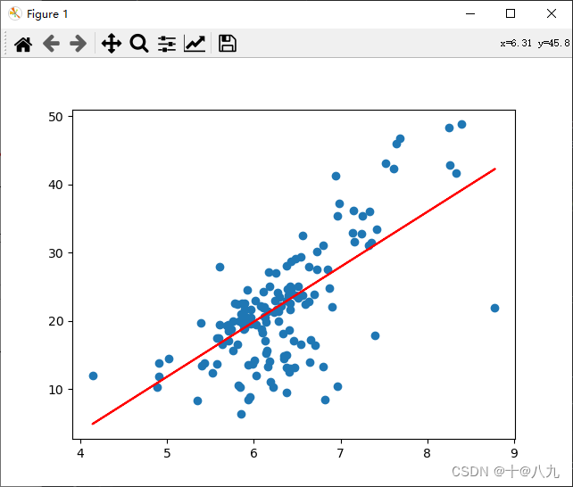
y_predict = lin_reg.predict(x_test.reshape(-1,1))
plt.scatter(x_test, y_test)
plt.plot(x_test, y_predict, c='r')
plt.show()# 获取相关参数:
# 斜率(coefficient):使用coef_属性
# 截距(intercept):使用intercept_属性
slope = lin_reg.coef_[0]
intercept = lin_reg.intercept_# 输出线性回归模型的斜率和截距,和回归方程式
print("斜率(coefficient):", slope)
print("截距(intercept):", intercept)
print(f'回归(拟合)方程式为: y={slope:.1f}*x + {intercept:.1f}')
斜率(coefficient): 8.056822140369604
截距(intercept): -28.493068724477876
回归(拟合)方程式为: y=8.1*x + -28.5
4 多元线性回归公式
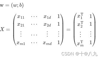
w ^ ∗ = ( X T X ) − 1 X T y {\hat w^*} = {({X^{\rm T}}X)^{ - 1}}{X^{\rm T}}y w^∗=(XTX)−1XTy
5 sklearn实现多元线性回归
注,线性回归中不需要归一化;sklearn实现的线性回归并非是4中的方法
import numpy as np
import pandas as pd
from matplotlib import pyplot as plt
from sklearn.model_selection import train_test_split
from sklearn.linear_model import LinearRegressiondata_url = "http://lib.stat.cmu.edu/datasets/boston"
raw_df = pd.read_csv(data_url, sep="\s+", skiprows=22, header=None)
data = np.hstack([raw_df.values[::2, :], raw_df.values[1::2, :2]])
target = raw_df.values[1::2, 2]
x = data
y = target
x = x[y<50]     # 该列数据的最大值是50,不移除的话会存在很多等于50的数据
y = y[y<50]lin_reg = LinearRegression()
x_train, x_test, y_train, y_test = train_test_split(x, y, test_size=0.3, random_state = 0)
lin_reg.fit(x_train, y_train)
y_predict = lin_reg.predict(x_test)
score = lin_reg.score(x_test, y_test)
print("score:", score)# 获取相关参数:
# 斜率(coefficient):使用coef_属性
# 截距(intercept):使用intercept_属性
slope = lin_reg.coef_[0]
intercept = lin_reg.intercept_
# 输出线性回归模型的斜率和截距,和回归方程式
print("coefficient:", slope)
print("intercept:", intercept)## 对比归一化后的效果
from sklearn.preprocessing import StandardScaler
standardScaler = StandardScaler()
standardScaler.fit(x_train)
x_train = standardScaler.transform(x_train)
x_test = standardScaler.transform(x_test)
lin_reg.fit(x_train, y_train)
score2 = lin_reg.score(x_test, y_test)
print("score2:", score)
score: 0.7455942658788959
coefficient: -0.12265382712227257
intercept: 35.07476409245881
score2: 0.7455942658788959
6 模型评价指标
M S E = 1 n ∑ i = 1 n ( y r e a l − y p r e d i c t ) 2 MSE = \frac{1}{n}\sum\limits_{i = 1}^n {{{({y_{real}} - {y_{predict}})}^2}} MSE=n1i=1∑n(yreal−ypredict)2
R M S E = 1 n ∑ i = 1 n ( y r e a l − y p r e d i c t ) 2 RMSE = \sqrt {\frac{1}{n}\sum\limits_{i = 1}^n {{{({y_{real}} - {y_{predict}})}^2}} } RMSE=n1i=1∑n(yreal−ypredict)2
M A E = 1 n ∣ y r e a l − y p r e d i c t ∣ MAE = \frac{1}{n}\left| {{y_{real}} - {y_{predict}}} \right| MAE=n1∣yreal−ypredict∣
R 2 = 1 − ∑ ( y r e a l − y p r e d i c t ) 2 ∑ ( y r e a l − y ˉ r e a l ) 2 = 1 − 1 n ∑ ( y r e a l − y p r e d i c t ) 2 1 n ( y r e a l − y ˉ r e a l ) 2 = 1 − M S E v a r ( y r e a l ) {R^2} = 1 - \frac{{\sum {{{({y_{real}} - {y_{predict}})}^2}} }}{{\sum {{{({y_{real}} - {{\bar y}_{real}})}^2}} }} = 1 - \frac{{\frac{1}{n}\sum {{{({y_{real}} - {y_{predict}})}^2}} }}{{\frac{1}{n}{{({y_{real}} - {{\bar y}_{real}})}^2}}} = 1 - \frac{{MSE}}{{{\mathop{\rm var}} ({y_{real}})}} R2=1−∑(yreal−yˉreal)2∑(yreal−ypredict)2=1−n1(yreal−yˉreal)2n1∑(yreal−ypredict)2=1−var(yreal)MSE
import numpy as np
import pandas as pd
import matplotlib.pyplot as plt
from sklearn.model_selection import train_test_split
from sklearn.linear_model import LinearRegression
import warnings
warnings.filterwarnings("ignore")data_url = "http://lib.stat.cmu.edu/datasets/boston"
raw_df = pd.read_csv(data_url, sep="\s+", skiprows=22, header=None)
data = np.hstack([raw_df.values[::2, :], raw_df.values[1::2, :2]])
target = raw_df.values[1::2, 2]
x = data[:, -1].reshape(-1, 1)
y = target.reshape(-1, 1)
x_train, x_test, y_train, y_test = train_test_split(x, y, test_size=0.3, random_state=0)linearReg = LinearRegression()
model = linearReg.fit(x_train, y_train)
y_predict = model.predict(x_test)
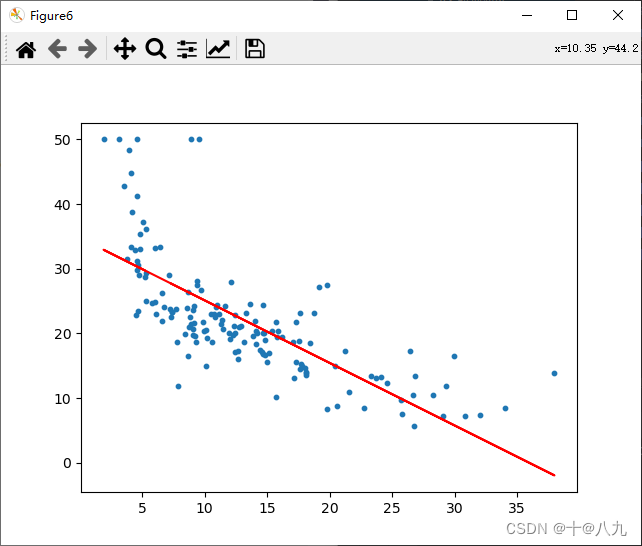
plt.figure(num='Figure6')
plt.scatter(x_test, y_test, s=10)
plt.plot(x_test, y_predict, c='r')
plt.show()y_real = y_test
# MSE
mse = np.sum((y_real - y_predict) ** 2) / len(y_test)
# RMSE
rmse = np.sqrt(mse)
# MAE
mae = np.sum(np.abs(y_real - y_predict)) / len(y_test)
# R2
r2 = 1 - (np.sum((y_real - y_predict) ** 2)) / (np.sum((y_real - np.mean(y_real)) ** 2))
r2_1 = 1 - mse / np.var(y_real)
print(f'MSE={mse:.1f}')
print(f'RMSE={rmse:.1f}')
print(f'MAE={mae:.1f}')
print(f'R2={r2:.3f}')
print(f'R2_1={r2_1:.3f}')
MSE=39.8
RMSE=6.3
MAE=4.5
R2=0.522
R2_1=0.522
上述评价指标也可用直接调用sklearn
# 接上面代码块
from sklearn.metrics import mean_squared_error
from sklearn.metrics import mean_absolute_error
from sklearn.metrics import r2_score# MSE
mse = mean_squared_error(y_real, y_predict)
# RMSE
rmse = mean_squared_error(y_real, y_predict, squared=False)
# MAE
mae = mean_absolute_error(y_real, y_predict)
# R2
r2 = r2_score(y_real, y_predict)
r2_1 = model.score(x_test, y_test)
print(f'MSE={mse:.1f}')
print(f'RMSE={rmse:.1f}')
print(f'MAE={mae:.1f}')
print(f'R2={r2:.3f}')
print(f'R2_1={r2_1:.3f}')
MSE=39.8
RMSE=6.3
MAE=4.5
R2=0.522
R2_1=0.522
回归模型中,损失函数一般使用MSE、RMSE、MAE,而性能评价指标多使用R2。
7 多项式回归
7.1将多项式回归作为线性回归处理
import numpy as np
import matplotlib.pyplot as plt
from sklearn.linear_model import LinearRegressionx = np.random.uniform(-4, 2, size=(100))
y = 2 * x ** 2 + 4 * x + 3 + np.random.randn(100)
X = x.reshape(-1, 1)
X_new = np.hstack([X, X ** 2])
linear_regression = LinearRegression()
linear_regression.fit(X_new, y)
y_predict = linear_regression.predict(X_new)
plt.scatter(x, y)
plt.plot(np.sort(x), y_predict[np.argsort(x)], color="red")
plt.show()# 输出线性回归模型的斜率和截距,和回归方程式
print("coefficient", linear_regression.coef_)
print("intercept", linear_regression.intercept_)
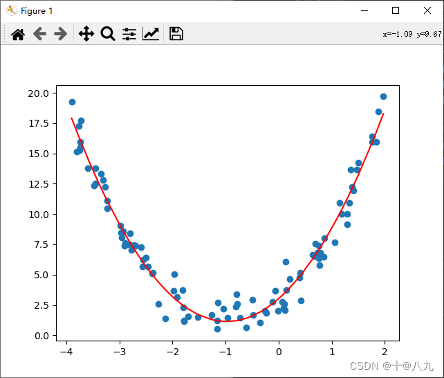
coefficient [3.84064494 1.9612757 ]
intercept 3.0225282289137976
7.2 sklaearn多项式特征维度扩展
import numpy as np
import matplotlib.pyplot as plt
from sklearn.preprocessing import PolynomialFeatures
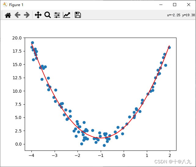
from sklearn.linear_model import LinearRegressionx = np.random.uniform(-4, 2, size=(100))
y = 2 * x ** 2 + 4 * x + 3 + np.random.randn(100)
X = x.reshape(-1, 1)
polynomial_features = PolynomialFeatures(degree=2)
X_poly = polynomial_features.fit_transform(X) # 二次多项式特征维度扩展
print(X_poly[:3])linear_regression = LinearRegression()
linear_regression.fit(X_poly, y)
y_predict = linear_regression.predict(X_poly)
plt.scatter(x, y)
plt.plot(np.sort(x), y_predict[np.argsort(x)], color="red")
plt.show()# 输出线性回归模型的斜率和截距,和回归方程式
print("coefficient", linear_regression.coef_)
print("intercept", linear_regression.intercept_)
[[ 1. -0.61108249 0.37342182]
[ 1. 0.70522585 0.4973435 ]
[ 1. -0.84277066 0.71026238]]
coefficient [0. 3.9052941 1.96796747]
intercept 3.056164951792293