本文结合实例详细讲解了如何使用Python对栅格数据进行地理加权回归(GWR)和多尺度地理加权回归分析(MGWR),关注公众号GeodataAnalysis,回复20230605获取示例数据和代码,包含整体的写作思路,上手运行一下代码更容易弄懂。
进行GWR和MGWR的工具有很多,但一般只针对矢量数据。对栅格数据进行GWR和MGWR分析,一般是将其转为矢量,计算后将结果再转为栅格。但在过程中比较容易出现各种问题,比如在一个像元上,有的指标是空值,有的不是,筛选起来就比较麻烦。用代码来做就比较灵活,且计算速度较快,因为栅格数据一般数据量比矢量大得多,计算起来就很复杂。
一、GWR和MGWR简介
地理加权回归 (GWR) 是若干空间回归技术中的一种,越来越多地用于地理及其他学科。通过使回归方程适合数据集中的每个要素,GWR 可为您要尝试了解/预测的变量或过程提供局部模型。GWR 构建这些独立方程的方法是:将落在每个目标要素的带宽范围内的要素的因变量和解释变量进行合并。带宽的形状和大小取决于用户输入的核类型、带宽方法、距离以及相邻点的数目参数。
MGWR 以地理加权回归 (GWR) 为基础构建。 它是一种局部回归模型,允许解释变量的系数随空间变化。 每个解释变量都可以在不同的空间尺度上运行。 GWR 不考虑这一点,但 MGWR 通过针对每个解释变量允许不同的邻域(带宽)来考虑这一点。 解释变量的邻域(带宽)将决定用于评估适合目标要素的线性回归模型中该解释变量系数的要素。

二、数据简介
因变量数据,2016年全国的PM2.5反演数据,空间分辨率为0.1度,开源于Surface PM2.5 | Atmospheric Composition Analysis Group | Washington University in St. Louis,简称为GWRPM25。
自变量数据,2016年全国的人为前体物排放数据,空间分辨率为0.25度,来源于清华大学MEIC(中国多尺度排放清单模型,Multi-resolution Emission Inventory for China,简称MEIC),本次使用CO、NOx、PM25、VOC四个指标。
三、数据预处理
NC数据转TIF
自变量数据和因变量数据都是NC格式,需要将其转为TIF,方便后续处理,更多的NC数据处理技巧参见公众号NetCDF(nc)读写与格式转换介绍一文。
MEIC数据转TIF
import os
import numpy as np
from netCDF4 import Dataset
from rasterio.crs import CRS
from rasterio.transform import from_bounds# MEIC数据的坐标、空间参考、nodata信息
west, south, east, north = 70, 10, 150, 60
width, height = 320, 200
meic_affine = from_bounds(west, south, east, north, width, height)
crs = CRS.from_epsg(4326)
nodata = -9999factors = ['CO', 'NOx', 'PM25', 'VOC']for factor in factors:factor_path = os.path.join('./meic_nc/', f'2016_00_total_{factor}.nc')out_path = os.path.join('./meic_tif/', f'{factor}.tif')ds = Dataset(factor_path)array = ds['z'][...].reshape(height, width)with rio.open(out_path, 'w', driver='GTiff', height=height, width=width, count=1, dtype=array.dtype, crs=crs, transform=meic_affine, nodata=nodata, compress='lzw') as dst:# 写入数据到输出文件dst.write(array, 1)
GWRPM25数据转TIF
x_res, y_res = 0.1, 0.1nc_path = './gwrpm25_nc/V5GL03.HybridPM25c_0p10.China.201601-201612.nc'
tif_path = './gwrpm25_tif/gwrpm25.tif'rootgrp = Dataset(nc_path)
# 获取分辨率和左上角像素坐标值
lon = rootgrp['lon'][...].data
lat = rootgrp['lat'][...].data
width, height = len(lon), len(lat)west, north = lon.min(), lat.max()
east = west + x_res * width
south = north - y_res * height
gwrpm25_affine = from_bounds(west, south, east, north, width, height)# 读取数据
pm = rootgrp['GWRPM25'][::-1, :]
pm = pm.filled(np.nan)with rio.open(tif_path, 'w', driver='GTiff', height=height, width=width, count=1, dtype=pm.dtype, crs=crs, transform=gwrpm25_affine, nodata=np.nan, compress='lzw') as dst:# 写入数据到输出文件dst.write(pm, 1)
GWRPM25数据重采样
由于自变量和因变量数据的空间范围以及分辨率不同,因此对GWRPM25数据进行重采样,采样到和MEIC相同的分辨率和空间范围。
from rasterio.warp import reprojectout_path = './gwrpm25_tif/gwrpm25_res.tif'
dst_array = np.empty((200, 320), dtype=np.float32)
reproject(# 源文件参数source=pm,src_crs=crs,src_transform=gwrpm25_affine, src_nodata=np.nan, # 目标文件参数destination=dst_array, dst_crs=crs, dst_transform=meic_affine,dst_nodata=np.nan
)
with rio.open(out_path, 'w', driver='GTiff', height=200, width=320, count=1, dtype=dst_array.dtype, crs=crs, transform=meic_affine, nodata=np.nan, compress='lzw') as dst:# 写入数据到输出文件dst.write(dst_array, 1)
四、GWR和MGWR分析
数据读取
用于计算多个栅格数据的共同非空值的掩膜。
def rasters_mask(paths):out_mask = Nonefor path in paths:src = rio.open(path)array = src.read(1)mask = ~(array==src.nodata)mask = mask & (~np.isnan(array))if isinstance(out_mask, type(None)):out_mask = maskelse:out_mask = out_mask & maskreturn out_mask
用于读取多个栅格数据返回Nmupy数组,mask参数指上一步计算的掩膜,结果数组形状为(n, k),n为有效样本点数量,k为paths的长度。
def rasters_to_array(paths, mask):out_array = Nonefor path in paths:src = rio.open(path)array = src.read(1)array = array.astype(np.float32)array = array[mask][..., np.newaxis]if isinstance(out_array, type(None)):out_array = arrayelse:out_array = np.concatenate([out_array, array], axis=1)return out_array
计算自变量和因变量的非空数据的掩膜。
x_paths = glob('./meic_tif/*.tif')
y_path = './gwrpm25_tif/gwrpm25_res.tif'
mask = rasters_mask(x_paths + [y_path])
获取自变量和因变量的有效像元值,有效栅格像元数越多后面计算GWR就越慢,指数级上升。
x_array = rasters_to_array(x_paths, mask)
y_array = rasters_to_array([y_path], mask)assert np.any(np.isnan(x_array)) == False
assert np.any(np.isnan(y_array)) == False
计算有效栅格像元的坐标
以栅格像元中心点的坐标作为这个像元的坐标。
src_y = rio.open('./gwrpm25_tif/gwrpm25_res.tif')
gt = src_y.transform
w, h = src_y.width, src_y.heightx_coords = np.arange(gt[2] + gt[0] / 2, gt[2] + gt[0] * w, gt[0])
y_coords = np.arange(gt[5] + gt[4] / 2, gt[5] + gt[4] * h, gt[4])
x_coords, y_coords = np.meshgrid(x_coords, y_coords)
x_coords, y_coords = x_coords[mask][..., np.newaxis], y_coords[mask][..., np.newaxis]
coords = np.concatenate([x_coords, y_coords], axis=1)
GWR分析
计算最佳带宽
# Reference:https://www.osgeo.cn/pysal/generated/pysal.model.mgwr.sel_bw.Sel_BW.html
pool = multiprocessing.Pool(processes = 6)
bw = Sel_BW(coords, y_array, x_array, kernel='gaussian').search(criterion='AIC', pool=pool)
拟合模型,输出结果中x0是偏置,x1 - x4是meic_tif文件夹中的四个指标,按文件名排序。
model = GWR(coords, y_array, x_array, bw=bw, fixed=False, kernel='gaussian')
results = model.fit(pool=pool)
results.summary()
Geographically Weighted Regression (GWR) Results
---------------------------------------------------------------------------
Spatial kernel:                                           Adaptive gaussian
Bandwidth used:                                                      51.000Diagnostic information
---------------------------------------------------------------------------
Residual sum of squares:                                         523320.602
Effective number of parameters (trace(S)):                          431.288
Degree of freedom (n - trace(S)):                                 15437.712
Sigma estimate:                                                       5.822
Log-likelihood:                                                  -50254.773
AIC:                                                             101374.121
AICc:                                                            101398.390
BIC:                                                             104690.685
R2:                                                                   0.926
Adjusted R2:                                                          0.923
Adj. alpha (95%):                                                     0.001
Adj. critical t value (95%):                                          3.442Summary Statistics For GWR Parameter Estimates
---------------------------------------------------------------------------
Variable                   Mean        STD        Min     Median        Max
-------------------- ---------- ---------- ---------- ---------- ----------
X0                       29.116     17.280      1.421     29.020     93.703
X1                        0.008      0.178     -2.029      0.000      1.861
X2                        0.000      0.353     -3.712     -0.001      4.119
X3                       -0.078      1.161    -13.198      0.000      8.369
X4                       -0.010      0.119     -1.729     -0.001      1.479
===========================================================================
MGWR分析
计算最佳带宽
# 数据量大,计算带宽太慢,MGWR不再演示
pool = multiprocessing.Pool(processes = 6)
selector = Sel_BW(coords, y_array, x_array, multi=True)
# multi_bw_min为搜索带宽的最小间隔,数据量小时可以设置大点
selector.search(multi_bw_min=[10], pool=pool)
拟合模型
model = MGWR(coords, y_array, x_array, selector, fixed=False, kernel='bisquare', sigma2_v1=True)
results = model.fit(pool=pool)
results.summary()
保存计算结果
以下结果为各指标的回归系数,bias表示偏置项。标度方差-协方差矩阵的保存方法与之相同,results.params替换为results.CCT即可。
factors = ['bias', 'CO', 'NOx', 'PM25', 'VOC']
result_params = results.params
for i, factor in enumerate(factors):factor_params = np.full(mask.shape, fill_value=np.nan, dtype=np.float32)factor_params[mask] = result_params[:, i]out_path = f'./results/{factor}.tif'with rio.open(out_path, 'w', driver='GTiff', height=factor_params.shape[0], width=factor_params.shape[1], count=1, dtype=factor_params.dtype, crs=src_y.crs, transform=src_y.transform, nodata=np.nan, compress='lzw') as dst:# 写入数据到输出文件dst.write(factor_params, 1)
以下结果为各个栅格像元的残差.
resid_response = np.full(mask.shape, fill_value=np.nan, dtype=np.float32)
resid_response[mask] = results.resid_response
out_path = f'./results/resid_response.tif'
with rio.open(out_path, 'w', driver='GTiff', height=resid_response.shape[0], width=resid_response.shape[1], count=1, dtype=resid_response.dtype, crs=src_y.crs, transform=src_y.transform, nodata=np.nan, compress='lzw') as dst:# 写入数据到输出文件dst.write(resid_response, 1)
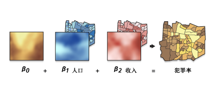
五、结果展示
各自变量指标的回归系数。