文章目录
- 前言
- 一、简单示例
- 二、gismo-3维IGA
- 3维程序中的几何模型
- 三、xml文件的理解
- 1、xml文件示例
- 2、gismo中二维示例文件-一个曲面(简单)
- 四、三维程序中xml文件的理解
- 三维几何模型
- 边界信息
- 五、三维程序运行
- 细化四次
- 细化5次
- 总结 #pic_center
前言
只是为方便学习,不做其他用途!
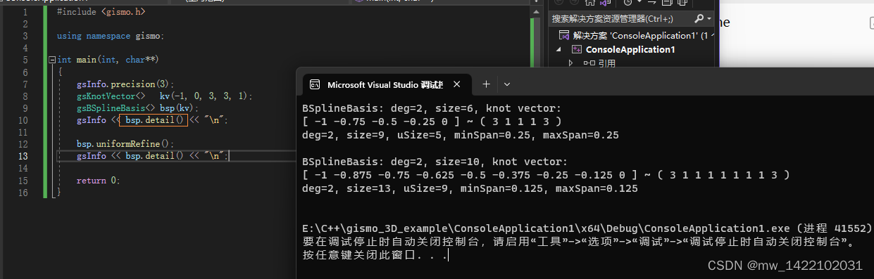
一、简单示例
参考网页 Tutorial 02: Geometry
#include <gismo.h>using namespace gismo;int main(int, char**)
{gsInfo.precision(3);gsKnotVector<>   kv(-1, 0, 3, 3, 1);gsBSplineBasis<> bsp(kv);gsInfo << bsp.detail() << "\n";bsp.uniformRefine();gsInfo << bsp.detail() << "\n";return 0;
}
二、gismo-3维IGA
运行代码需要配置好gismo环境
还需要将 terrific.xml 放在项目文件下,和cpp文件放在同一文件路径下

/// This is an example of using the linear elasticity solver on a 3D multi-patch geometry.
/// The problems is part of the EU project "Terrific".
///
/// Authors: O. Weeger (2012-1015, TU Kaiserslautern),
///          A.Shamanskiy (2016 - ...., TU Kaiserslautern)
#include <gismo.h>
#include <gsElasticity/gsElasticityAssembler.h>
#include <gsElasticity/gsWriteParaviewMultiPhysics.h>
#include <gsElasticity/gsGeoUtils.h>using namespace gismo;int main(int argc, char* argv[])
{gsInfo << "Testing the linear elasticity solver in 3D-线弹性求解器的三维测试.\n";//=============================================================//// Input ////=============================================================////std::string filename("terrific.xml");//初始数据文件std::string filename("test.xml");//初始数据文件real_t youngsModulus = 74e9;//杨氏模量real_t poissonsRatio = 0.33;//泊松比index_t numUniRef = 0;//节点插入数index_t numDegElev = 0;//升阶次数index_t numPlotPoints = 10000;//preview软件画图的点数量// minimalistic user interface for terminal 终端最简用户界面gsCmdLine cmd("Testing the linear elasticity solver in 3D.");// 定义一个gsCmdLine类 命名为cmdcmd.addInt("r", "refine", "Number of uniform refinement application", numUniRef);cmd.addInt("d", "degelev", "Number of degree elevation application", numDegElev);cmd.addInt("p", "points", "Number of points to plot to Paraview", numPlotPoints);try { cmd.getValues(argc, argv); } //  不太用看  不知道这个命令代表啥catch (int rv) { return rv; }//=====================================================================//// Scanning geometry and creating bases:扫描几何和创建基函数  ////=====================================================================//// scanning geometry 扫描几何gsMultiPatch<> geometry; //  定义一个多片gsReadFile<>(filename, geometry);// 将plateWithHole.xml文件中的数据赋值给 geometry// creating basis 生成基函数gsMultiBasis<> basis(geometry);for (index_t i = 0; i < numDegElev; ++i) // 升阶次数basis.degreeElevate();for (index_t i = 0; i < numUniRef; ++i) // k细化(节点插入)次数basis.uniformRefine();gsInfo << basis ;//=====================================================================//// Setting loads and boundary conditions  设置载荷和边界条件 ////=====================================================================//// source function, rhs  源函数?-解析解?gsConstantFunction<> f(0., 0., 0., 3);// surface load, neumann BC 黎曼边界对应载荷边界条件  荷载BC   力的边界条件gsConstantFunction<> g(20e6, -14e6, 0, 3);// boundary conditions 边界条件  黎曼边界对应载荷边界条件    dirichlete对应位移边界条件gsBoundaryConditions<> bcInfo;// Dirichlet BC are imposed separately for every component (coordinate) 对每个分量(坐标)分别施加 Dirichlet BCfor (index_t d = 0; d < 3; d++){bcInfo.addCondition(0, boundary::back, condition_type::dirichlet, 0, d);/* bcInfo.addCondition(1, boundary::back, condition_type::dirichlet, 0, d);bcInfo.addCondition(2, boundary::south, condition_type::dirichlet, 0, d);*/}// Neumann BC are imposed as one function 将 Neumann BC 作为一个函数bcInfo.addCondition(0, boundary::front, condition_type::neumann, &g);//bcInfo.addCondition(14, boundary::north, condition_type::neumann, &g);//=====================================================================//// Assembling & solving ////=====================================================================//// creating assembler   创建刚度矩阵?gsElasticityAssembler<real_t> assembler(geometry, basis, bcInfo, f);assembler.options().setReal("YoungsModulus", youngsModulus);assembler.options().setReal("PoissonsRatio", poissonsRatio);assembler.options().setInt("DirichletValues", dirichlet::l2Projection);gsInfo << "Assembling...\n";gsStopwatch clock;clock.restart();assembler.assemble();gsInfo << "Assembled a system with "<< assembler.numDofs() << " dofs in " << clock.stop() << "s.\n";gsInfo << "Solving...\n";clock.restart();#ifdef GISMO_WITH_PARDISOgsSparseSolver<>::PardisoLDLT solver(assembler.matrix());gsVector<> solVector = solver.solve(assembler.rhs());gsInfo << "Solved the system with PardisoLDLT solver in " << clock.stop() << "s.\n";
#elsegsSparseSolver<>::SimplicialLDLT solver(assembler.matrix());gsVector<> solVector = solver.solve(assembler.rhs());gsInfo << "Solved the system with EigenLDLT solver in " << clock.stop() << "s.\n";
#endif//=====================================================================//// Output ////=====================================================================//// constructing solution as an IGA functiongsMultiPatch<> solution;assembler.constructSolution(solVector, assembler.allFixedDofs(), solution);// constructing stressesgsPiecewiseFunction<> stresses;assembler.constructCauchyStresses(solution, stresses, stress_components::von_mises);if (numPlotPoints > 0){// constructing an IGA field (geometry + solution)gsField<> solutionField(assembler.patches(), solution);gsField<> stressField(assembler.patches(), stresses, true);// creating a container to plot all fields to one Paraview filestd::map<std::string, const gsField<>*> fields;fields["Deformation"] = &solutionField;fields["von Mises"] = &stressField;gsWriteParaviewMultiPhysics(fields, "test_le", numPlotPoints);gsInfo << "Open \"test_le.pvd\" in Paraview for visualization.\n";}return 0;
}
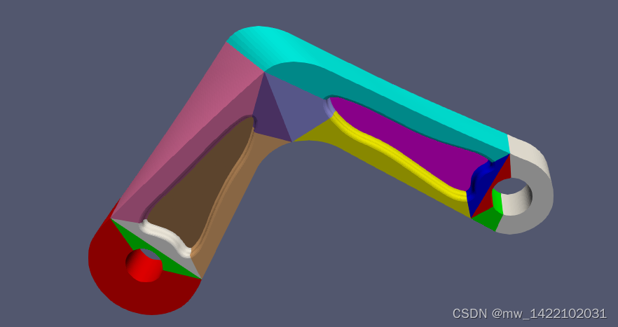
3维程序中的几何模型

三、xml文件的理解
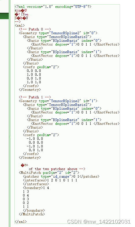
1、xml文件示例
网址https://gismo.github.io/Tutorial02.html

2、gismo中二维示例文件-一个曲面(简单)
可以参考之前的博客gismo中用等几何解决线弹性问题的程序示例来理解xml文件
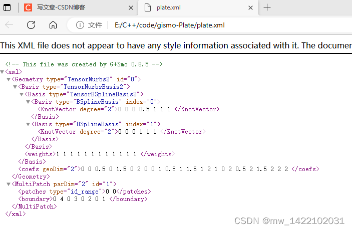

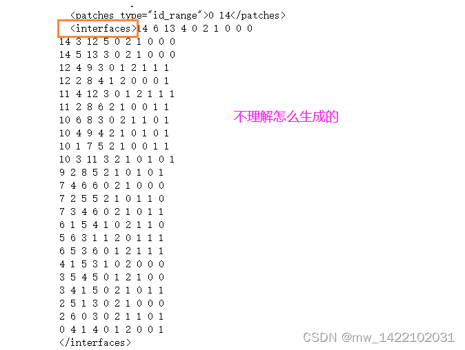
注: 一个平面没有 interfaces这一项
对 interfaces这一项 目前还没有理解
四、三维程序中xml文件的理解
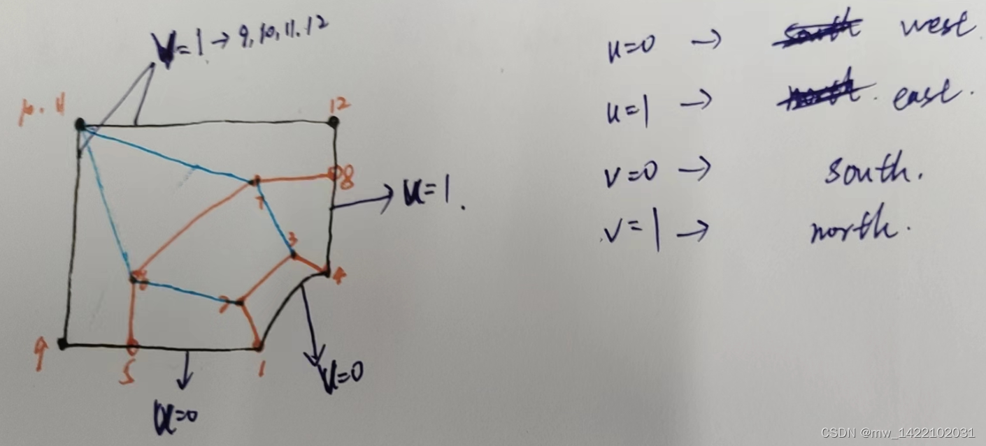
三维几何模型
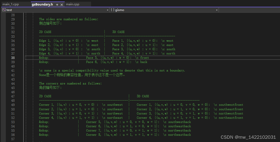
边界信息
给的示例文件中有15个体组装在一起


五、三维程序运行
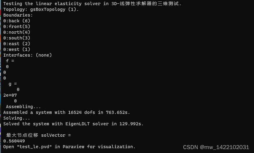
细化四次
运行时间:14分钟
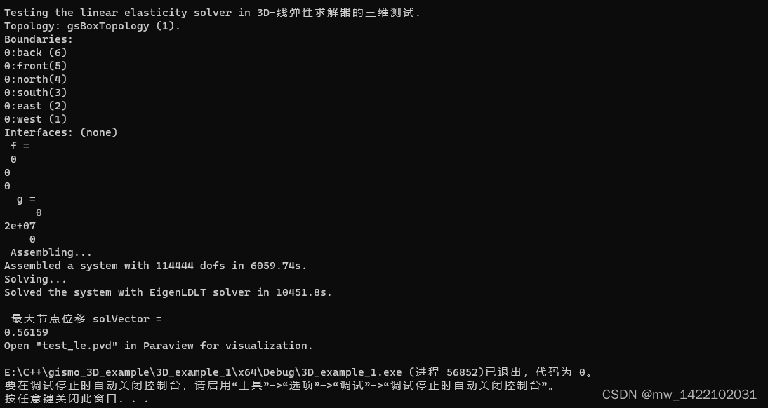
细化5次
运行时间:4.58h
组总刚:1.6h
解方程组:2.98h
总结 #pic_center
空格 空格
:
| 二维数 |
| 1 |
| 1 |
| 1 |
![[AHK]获取通达信软件上的股票代码](https://img-blog.csdnimg.cn/20200206142713553.png?x-oss-process=image/watermark,type_ZmFuZ3poZW5naGVpdGk,shadow_10,text_aHR0cHM6Ly9ibG9nLmNzZG4ubmV0L2xpdXl1a3Vhbg==,size_16,color_FFFFFF,t_70)