🤵♂️ 个人主页:@艾派森的个人主页
✍🏻作者简介:Python学习者
🐋 希望大家多多支持,我们一起进步!😄
如果文章对你有帮助的话,
欢迎评论 💬点赞👍🏻 收藏 📂加关注+
目录
1.项目背景
2.数据集介绍
3.技术工具
4.实验过程
4.1导入数据
4.2数据预处理
4.3数据可视化
4.4特征工程
4.5模型构建
4.6模型评估
5.总结
源代码
1.项目背景
能源价格的预测一直是经济领域中的一个重要问题,对于能源市场的参与者以及相关产业的发展都具有重要意义。随着能源市场的复杂性和不确定性不断增加,传统的经济模型在预测能源价格方面存在一定的局限性,因此需要引入更加灵活和准确的预测方法。
深度学习作为人工智能领域的一个重要分支,在处理时序数据和复杂特征方面具有优势。其中,循环神经网络(RNN)和卷积神经网络(CNN)是两种常用的深度学习模型,它们分别擅长处理序列数据和空间特征,可以有效地捕捉数据中的时序信息和空间关联。
结合RNN和CNN来预测能源价格具有一定的理论基础和实际应用前景。RNN可以很好地捕捉能源价格中的时序变化规律,例如季节性变化、周期性波动等,而CNN则可以有效地提取能源价格中的空间特征,例如不同地区之间的价格差异、价格分布的空间相关性等。将这两种模型结合起来,可以充分利用它们各自的优势,提高能源价格预测的准确性和稳定性。
因此,基于深度学习RNN和CNN的能源价格预测模型具有重要的研究意义和应用价值。通过构建和优化这样的预测模型,可以为能源市场的参与者提供更准确的价格预测信息,帮助其制定合理的决策和战略。同时,这也为深度学习在经济领域中的应用提供了一个重要的实证案例,对于推动深度学习在经济领域的进一步发展具有积极意义。
2.数据集介绍
数据集来源于Kaggle,原始数据集共有35064条,28个变量。在当今动态的能源市场中,准确预测能源价格对有效决策和资源配置至关重要。在这个项目中,我们使用先进的深度学习技术——特别是一维卷积神经网络(CNN)和循环神经网络(RNN)——深入研究预测分析领域。通过利用能源价格数据中的历史模式和依赖关系,我们的目标是建立能够高精度预测未来能源价格的模型。
3.技术工具
Python版本:3.9
代码编辑器:jupyter notebook
4.实验过程
4.1导入数据
导入第三方库并加载数据
import pandas as pd
import numpy as np
import matplotlib.pyplot as plt
import seaborn as sns
import warnings
warnings.filterwarnings('ignore')data = pd.read_csv('energy_dataset.csv', parse_dates = ['time'])
data.head()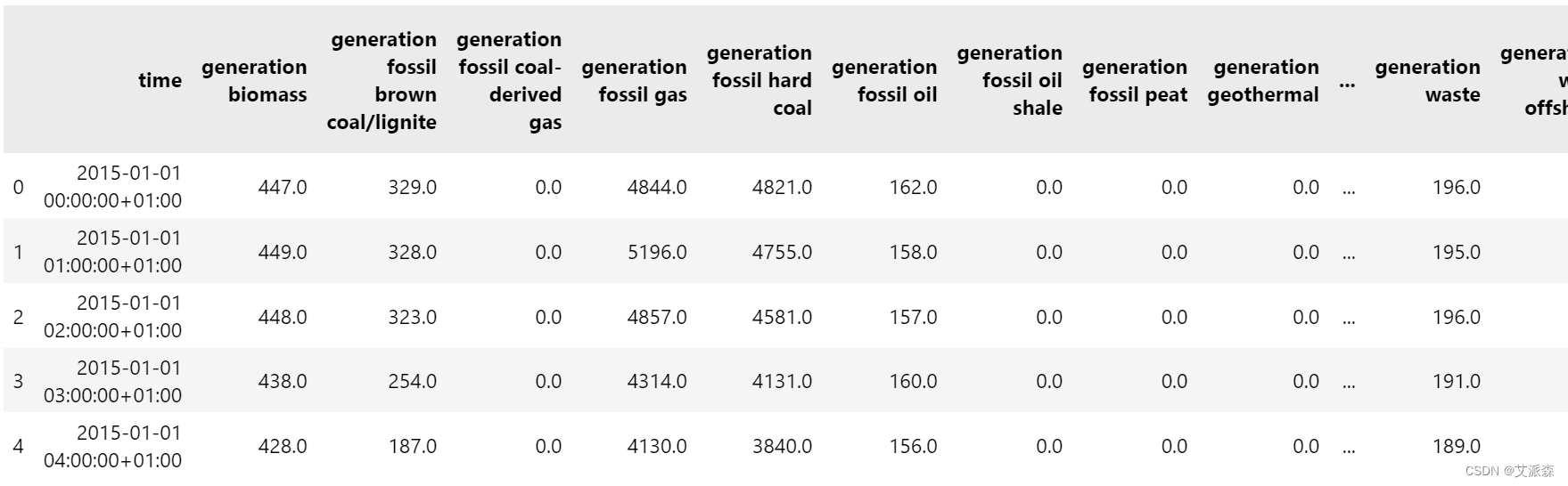
查看数据大小

4.2数据预处理
data.time = pd.to_datetime(data.time, utc = True, infer_datetime_format= True)
data = data.set_index('time')
data.head()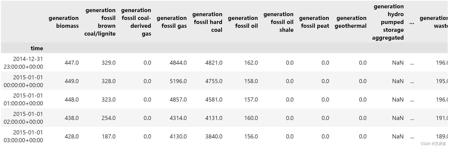
data.isnull().sum()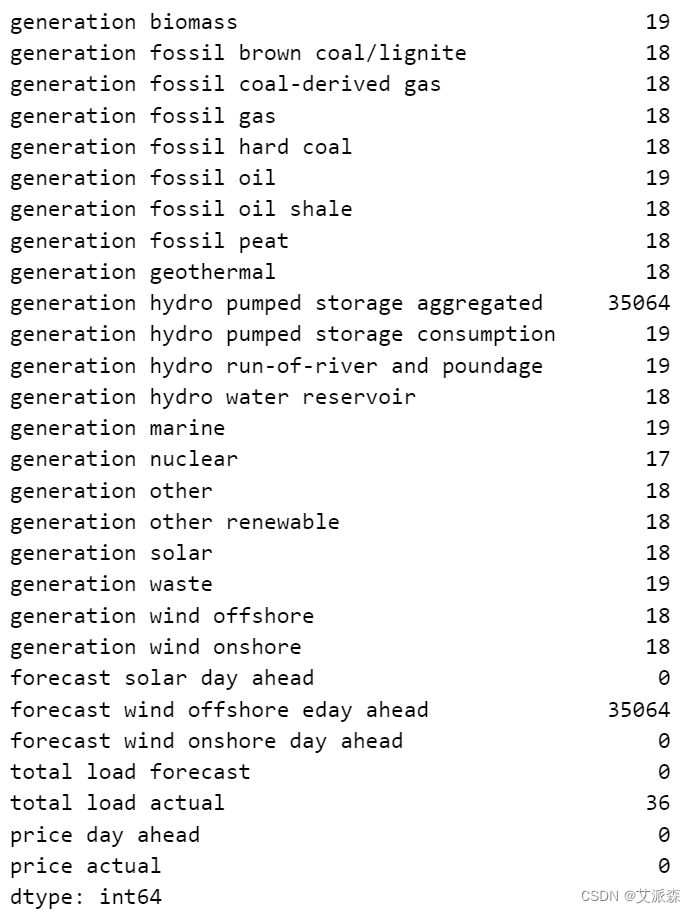
正如我们所看到的,在不同的列中有很多空行。所以我们必须处理好这个问题。
# 统计Dataframe所有列中0的个数
for column_name in data.columns:column = data[column_name]# 获取列中0的计数count = (column == 0).sum()print(f"{column_name:{50}} : {count}")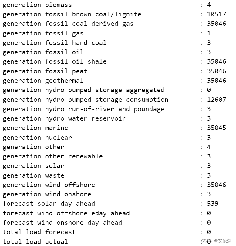
# 让我们删除不必要的列
data.drop(['generation hydro pumped storage aggregated', 'forecast wind offshore eday ahead','generation wind offshore', 'generation fossil coal-derived gas','generation fossil oil shale', 'generation fossil peat', 'generation marine','generation wind offshore', 'generation geothermal'], inplace = True, axis = 1)
data.isnull().sum()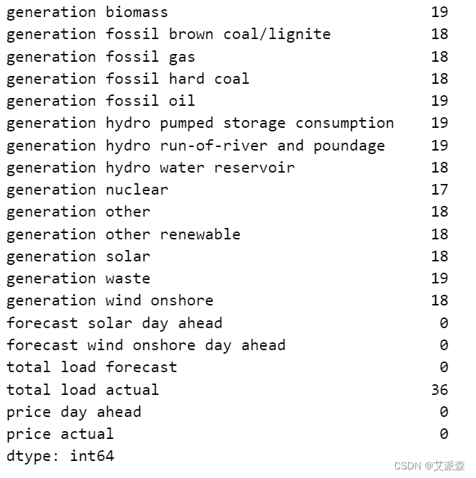
plt.rcParams['figure.figsize'] = (15, 5)
plt.plot(data['total load actual'][:24*7*2])
plt.show()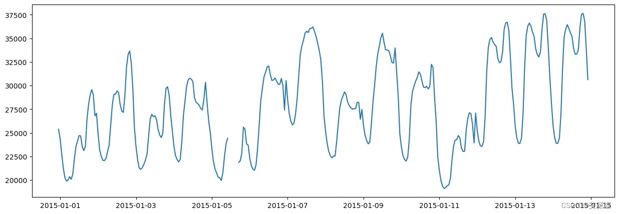
# 线性插值数据集中缺失的值
data.interpolate(method='linear', limit_direction='forward', inplace=True, axis=0)
data.isnull().sum()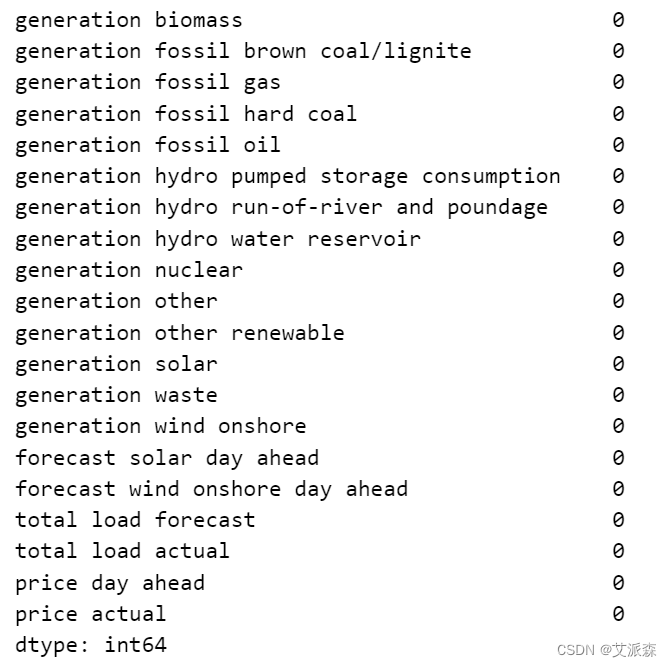
# 创建一个新列来计算总发电量
data['total generation'] = data['generation biomass'] + data['generation fossil brown coal/lignite'] + data['generation fossil gas'] + data['generation fossil hard coal'] + data['generation fossil oil'] + data['generation hydro pumped storage consumption'] + data['generation hydro run-of-river and poundage'] + data['generation hydro water reservoir'] + data['generation nuclear'] + data['generation other'] + data['generation other renewable'] + data['generation solar'] + data['generation waste'] + data['generation wind onshore']
data.head()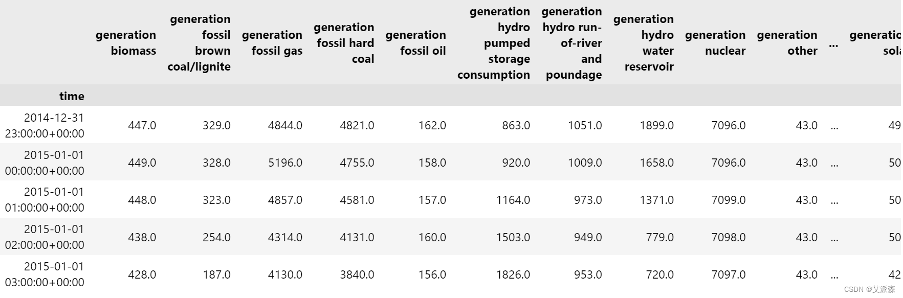
4.3数据可视化
sns.distplot(x=data['total generation'], kde=True, hist=True, hist_kws={'alpha': 0.5})
plt.show()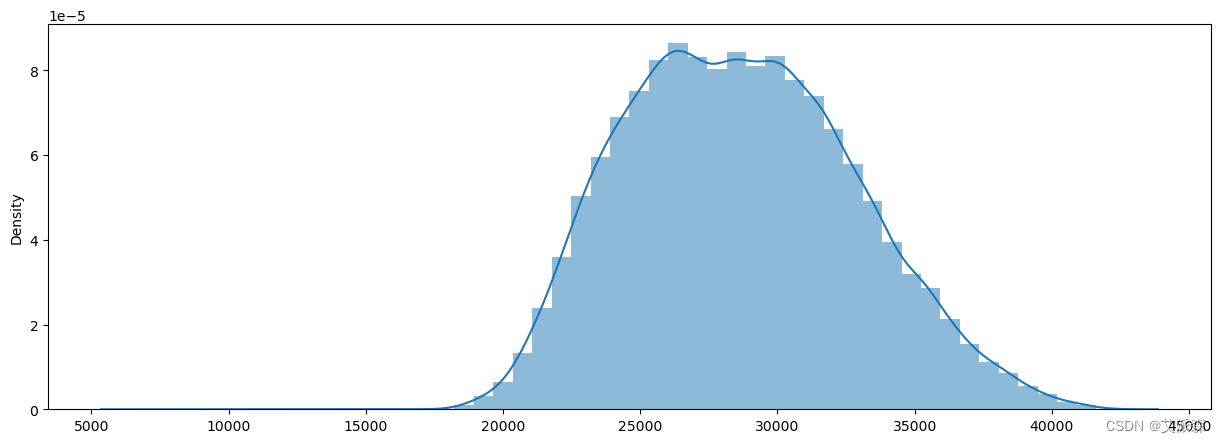
# 绘制一周内每小时的实际电价及其滚动平均值
fig, ax = plt.subplots(1, 1)
rolling = data['price actual'].rolling(24*7, center=True).mean()
ax.plot(data['price actual'], color='#4CAF50', label='Actual Price', marker='o', markersize=3)
ax.plot(rolling, color='#2196F3', linestyle='-', linewidth=2, label='Weekly Rolling Mean')
ax.grid(True)
plt.legend(fontsize='large')
plt.title('Hourly Electricity Price and Weekly Rolling Mean')
plt.xlabel('Time')
plt.ylabel('Price')
plt.tight_layout()
plt.show()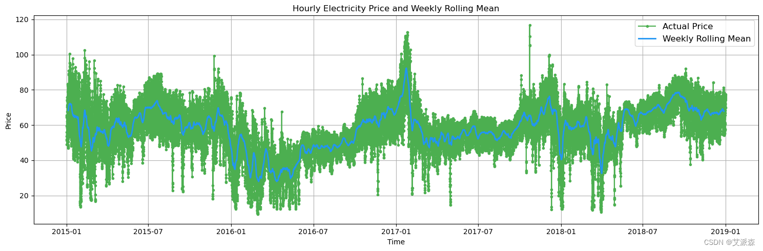
# 绘制电价(按月计算)以及第一年的滞后
monthly_price = data['price actual'].asfreq('M')
lagged = monthly_price.shift(12)
fig, ax = plt.subplots(1, 1)
ax.plot(monthly_price, label='Monthly Price', color='#4CAF50', linewidth=2)
ax.plot(lagged, label='1 yr lagged', color='#2196F3', linewidth=2)
ax.grid(True)
plt.legend(fontsize='large')
plt.title('Electricity Price (Month-wise) with 1st Year Lag')
plt.xlabel('Time (Months)')
plt.ylabel('Price')
plt.show()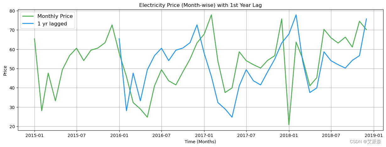
由于我们可以在两个图中看到类似的峰值,我们可以说数据中存在一些季节性模式。
# 绘制3周的每小时数据
start = 1+ 24*300
end = 1+ 24*322
plt.plot(data['price actual'][start:end])
plt.show()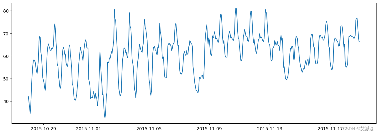
sns.distplot(x = data['price actual'], kde = True)
plt.show()
结论:价格服从正态分布。
4.4特征工程
# 拆分数据集
def prepare_dataset(data, size):x_data = []y_data = []l = len(data) - sizefor i in range(l):x = data[i:i+size]y = data[i+size]x_data.append(x)y_data.append(y)return np.array(x_data), np.array(y_data)# 为plot创建函数,我们稍后会用到它
def plot_model_rmse_and_loss(history, title):# 评估训练和验证的准确性和损失train_rmse = history.history['root_mean_squared_error']val_rmse = history.history['val_root_mean_squared_error']train_loss = history.history['loss']val_loss = history.history['val_loss']plt.figure(figsize=(15, 5))# 绘制训练和验证RMSEplt.subplot(1, 2, 1)plt.plot(train_rmse, label='Training RMSE', color='blue', linestyle='-')plt.plot(val_rmse, label='Validation RMSE', color='orange', linestyle='--')plt.xlabel('Epochs')plt.ylabel('RMSE')plt.title('Epochs vs. Training and Validation RMSE')plt.legend()# 绘图训练和验证损失plt.subplot(1, 2, 2)plt.plot(train_loss, label='Training Loss', color='green', linestyle='-')plt.plot(val_loss, label='Validation Loss', color='red', linestyle='--')plt.xlabel('Epochs')plt.ylabel('Loss')plt.title('Epochs vs. Training and Validation Loss')plt.legend()plt.suptitle(title, fontweight='bold', fontsize=15)# 调整布局以防止元素重叠plt.tight_layout()plt.show()
# 标准化处理
from sklearn.preprocessing import MinMaxScaler
data_filtered = data['price actual'].values
scaler = MinMaxScaler(feature_range = (0,1))
scaled_data = scaler.fit_transform(data_filtered.reshape(-1,1))
scaled_data.shape 
# 查看训练集和测试集大小
train_size = int(np.ceil(len(scaled_data) * 0.8))
test_size = int((len(scaled_data) - train_size) *0.5)
print(train_size, test_size)
# 拆分数据集为训练集、测试集、验证集
xtrain, ytrain = prepare_dataset(scaled_data[:train_size], 25)
xval, yval = prepare_dataset(scaled_data[train_size-25:train_size +test_size], 25)
xtest, ytest = prepare_dataset(scaled_data[train_size + test_size-25:], 25)
print(xtrain.shape)
print(xval.shape)
print(xtest.shape)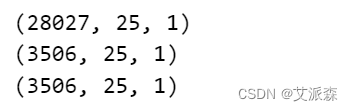
4.5模型构建
导入第三方库
import tensorflow as tf
from tensorflow.keras import Sequential
from tensorflow.keras.layers import Dense, LSTM, Dropout, Conv1D, Flatten, SimpleRNN
loss = tf.keras.losses.MeanSquaredError()
metric = [tf.keras.metrics.RootMeanSquaredError()]
optimizer = tf.keras.optimizers.Adam()
early_stopping = [tf.keras.callbacks.EarlyStopping(monitor = 'loss', patience = 5)]第一种方法:堆叠SimpleRNN
# 第一种方法:堆叠SimpleRNN
# Create a Sequential model (a linear stack of layers)
model_SimpleRNN = Sequential()# Add a SimpleRNN layer with 128 units and return sequences for the next layer
# input_shape: Shape of input data (number of timesteps, number of features)
model_SimpleRNN.add(SimpleRNN(128, return_sequences=True, input_shape=(xtrain.shape[1], 1)))# Add another SimpleRNN layer with 64 units and do not return sequences
model_SimpleRNN.add(SimpleRNN(64, return_sequences=False))# Add a fully connected Dense layer with 64 units
model_SimpleRNN.add(Dense(64))# Add a Dropout layer with dropout rate of 0.2 to prevent overfitting
model_SimpleRNN.add(Dropout(0.2))# Add a fully connected Dense layer with 1 unit for regression
model_SimpleRNN.add(Dense(1))# Compile the model with specified loss function, evaluation metrics, and optimizer
model_SimpleRNN.compile(loss=loss, metrics=metric, optimizer=optimizer)# Train the model using training data (xtrain, ytrain) for a specified number of epochs
# Validate the model using validation data (xval, yval)
# early_stopping: A callback function to stop training if validation loss does not improve
history = model_SimpleRNN.fit(xtrain, ytrain, epochs=10, validation_data=(xval, yval), callbacks=early_stopping)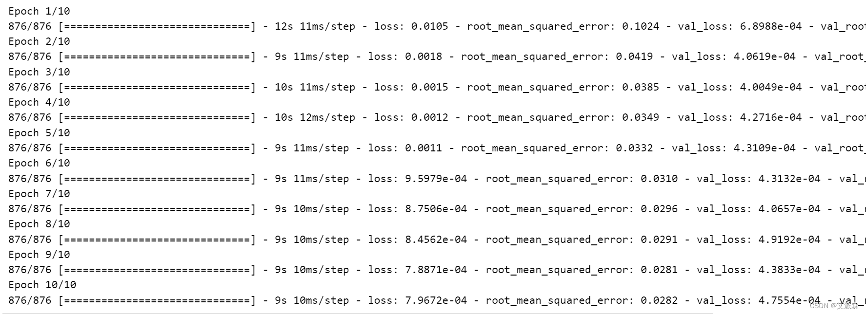
plot_model_rmse_and_loss(history,"SimpleRNN")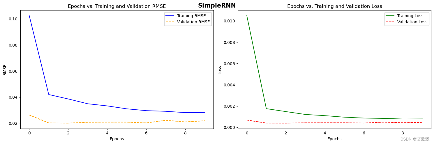
模型评估
# Generate predictions using the trained SimpleRNN model on the test data
predictions = model_SimpleRNN.predict(xtest)# Inverse transform the scaled predictions to the original scale using the scaler
predictions = scaler.inverse_transform(predictions)# Calculate the Root Mean Squared Error (RMSE) between the predicted and actual values
# RMSE is a commonly used metric to measure the difference between predicted and actual values
simplernn_rmse = np.sqrt(np.mean(((predictions - ytest) ** 2)))# Print the Root Mean Squared Error for SimpleRNN model
print(f"Root Mean Squared Error for SimpleRNN = {simplernn_rmse}")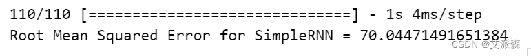
第二种方法:CNN 1D
# 第二种方法:CNN 1D
from tensorflow.keras.optimizers import Adam# Create a Sequential model (a linear stack of layers)
model_CNN = Sequential()# Add a 1D convolutional layer with 48 filters, kernel size of 2, 'causal' padding, and ReLU activation
# Input shape: Shape of input data (number of timesteps, number of features)
model_CNN.add(Conv1D(filters=48, kernel_size=2, padding='causal', activation='relu', input_shape=(xtrain.shape[1], 1)))# Flatten the output of the convolutional layer to be fed into the Dense layers
model_CNN.add(Flatten())# Add a fully connected Dense layer with 48 units and ReLU activation
model_CNN.add(Dense(48, activation='relu'))# Add a Dropout layer with dropout rate of 0.2 to prevent overfitting
model_CNN.add(Dropout(0.2))# Add a fully connected Dense layer with 1 unit for regression
model_CNN.add(Dense(1))# Use legacy optimizer tf.keras.optimizers.legacy.Adam with default learning rate
optimizer = Adam()# Compile the model with specified loss function, evaluation metrics, and optimizer
model_CNN.compile(loss=loss, metrics=metric, optimizer=optimizer)# Train the model using training data (xtrain, ytrain) for a specified number of epochs
# Validate the model using validation data (xval, yval)
# early_stopping: A callback function to stop training if validation loss does not improve
history = model_CNN.fit(xtrain, ytrain, epochs=10, validation_data=(xval, yval), callbacks=early_stopping)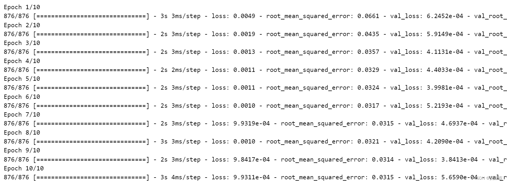
# Plot the RMSE and loss curves for the CNN 1D model using the training history
plot_model_rmse_and_loss(history, "CNN 1D")# Generate predictions using the trained CNN 1D model on the test data
predictions = model_CNN.predict(xtest)# Inverse transform the scaled predictions to the original scale using the scaler
predictions = scaler.inverse_transform(predictions)# Calculate the Root Mean Squared Error (RMSE) between the predicted and actual values
# RMSE is a commonly used metric to measure the difference between predicted and actual values
CNN_rmse = np.sqrt(np.mean(((predictions - ytest) ** 2)))# Print the Root Mean Squared Error for the CNN 1D model
print(f"\nRoot Mean Squared Error for CNN 1D = {CNN_rmse}")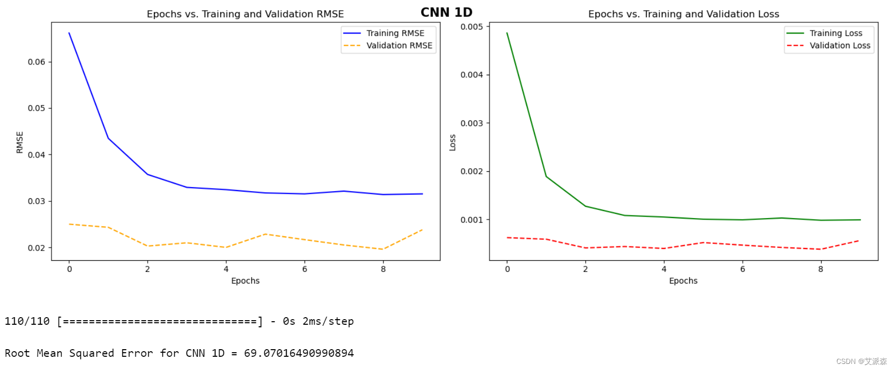
第三种方法:CNN-LSTM
# 第三种方法:CNN-LSTM
from tensorflow.keras.optimizers import Adam# Create a Sequential model for CNN-LSTM architecture
model_CNN_LSTM = Sequential()# Add a 1D convolutional layer with 100 filters, kernel size of 2, 'causal' padding, and ReLU activation
# Input shape: Shape of input data (number of timesteps, number of features)
model_CNN_LSTM.add(Conv1D(filters=100, kernel_size=2, padding='causal', activation='relu', input_shape=(xtrain.shape[1], 1)))# Add a Long Short-Term Memory (LSTM) layer with 100 units and return sequences
model_CNN_LSTM.add(LSTM(100, return_sequences=True))# Flatten the output of the LSTM layer to be fed into the Dense layers
model_CNN_LSTM.add(Flatten())# Add a fully connected Dense layer with 100 units and ReLU activation
model_CNN_LSTM.add(Dense(100, activation='relu'))# Add a Dropout layer with dropout rate of 0.2 to prevent overfitting
model_CNN_LSTM.add(Dropout(0.2))# Add a fully connected Dense layer with 1 unit for regression
model_CNN_LSTM.add(Dense(1))# Use legacy optimizer tf.keras.optimizers.legacy.Adam with default learning rate
optimizer = Adam()# Compile the model with specified loss function, evaluation metrics, and optimizer
model_CNN_LSTM.compile(loss=loss, metrics=metric, optimizer=optimizer)# Train the model using training data (xtrain, ytrain) for a specified number of epochs
# Validate the model using validation data (xval, yval)
# early_stopping: A callback function to stop training if validation loss does not improve
history = model_CNN_LSTM.fit(xtrain, ytrain, epochs=10, validation_data=(xval, yval), callbacks=early_stopping)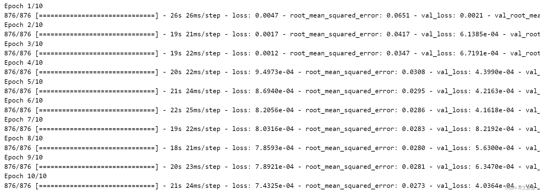
# Plot the RMSE and loss curves for the CNN-LSTM model using the training history
plot_model_rmse_and_loss(history, "CNN-LSTM")# Generate predictions using the trained CNN-LSTM model on the test data
predictions = model_CNN_LSTM.predict(xtest)# Inverse transform the scaled predictions to the original scale using the scaler
predictions = scaler.inverse_transform(predictions)# Calculate the Root Mean Squared Error (RMSE) between the predicted and actual values
# RMSE is a commonly used metric to measure the difference between predicted and actual values
CNN_LSTM_rmse = np.sqrt(np.mean(((predictions - ytest) ** 2)))
print(f"\nRoot Mean Squarred Error for CNN-LSTM = {CNN_LSTM_rmse}")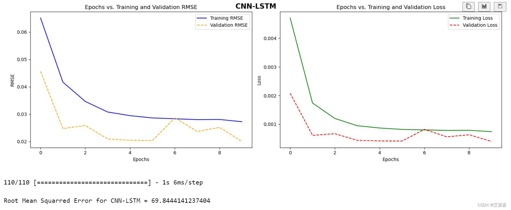
4.6模型评估
# Print the Root Mean Squared Error for SimpleRNN model
print(f"Root Mean Squared Error for SimpleRNN = {simplernn_rmse}")# Print the Root Mean Squared Error for CNN 1D model
print(f"Root Mean Squared Error for CNN 1D = {CNN_rmse}")# Print the Root Mean Squared Error for CNN-LSTM model
print(f"Root Mean Squared Error for CNN-LSTM = {CNN_LSTM_rmse}")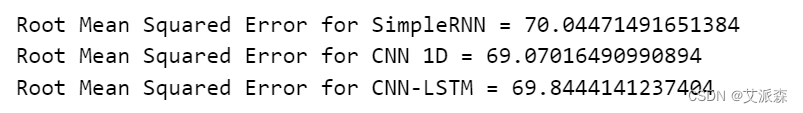
5.总结
通过实验,我们发现每种方法都有自己的优点和局限性。SimpleRNN提供了一个简单且可解释的体系结构,但可能会与长期依赖关系作斗争。1D CNN在捕获数据的局部模式和波动方面是有效的。CNN-LSTM结合了cnn和lstm的优点,为捕获短期和长期依赖提供了一个强大的框架。方法的选择取决于数据集的具体特征和手头的预测任务。
总之,我们对SimpleRNN、1D CNN和CNN- lstm模型的探索为它们在时间序列预测任务中的适用性和性能提供了有价值的见解。通过了解每种方法的优点和局限性,从业者可以在为他们的预测需求选择最合适的体系结构时做出明智的决定。
源代码
import pandas as pd
import numpy as np
import matplotlib.pyplot as plt
import seaborn as sns
import warnings
warnings.filterwarnings('ignore')data = pd.read_csv('energy_dataset.csv', parse_dates = ['time'])
data.head()
data.shape
data.time = pd.to_datetime(data.time, utc = True, infer_datetime_format= True)
data = data.set_index('time')
data.head()
data.isnull().sum()
正如我们所看到的,在不同的列中有很多空行。所以我们必须处理好这个问题
# 统计Dataframe所有列中0的个数
for column_name in data.columns:column = data[column_name]# 获取列中0的计数count = (column == 0).sum()print(f"{column_name:{50}} : {count}")
# 让我们删除不必要的列
data.drop(['generation hydro pumped storage aggregated', 'forecast wind offshore eday ahead','generation wind offshore', 'generation fossil coal-derived gas','generation fossil oil shale', 'generation fossil peat', 'generation marine','generation wind offshore', 'generation geothermal'], inplace = True, axis = 1)
data.isnull().sum()
plt.rcParams['figure.figsize'] = (15, 5)
plt.plot(data['total load actual'][:24*7*2])
plt.show()
# 线性插值数据集中缺失的值
data.interpolate(method='linear', limit_direction='forward', inplace=True, axis=0)
data.isnull().sum()
# 创建一个新列来计算总发电量
data['total generation'] = data['generation biomass'] + data['generation fossil brown coal/lignite'] + data['generation fossil gas'] + data['generation fossil hard coal'] + data['generation fossil oil'] + data['generation hydro pumped storage consumption'] + data['generation hydro run-of-river and poundage'] + data['generation hydro water reservoir'] + data['generation nuclear'] + data['generation other'] + data['generation other renewable'] + data['generation solar'] + data['generation waste'] + data['generation wind onshore']
data.head()
sns.distplot(x=data['total generation'], kde=True, hist=True, hist_kws={'alpha': 0.5})
plt.show()
# 绘制一周内每小时的实际电价及其滚动平均值
fig, ax = plt.subplots(1, 1)
rolling = data['price actual'].rolling(24*7, center=True).mean()
ax.plot(data['price actual'], color='#4CAF50', label='Actual Price', marker='o', markersize=3)
ax.plot(rolling, color='#2196F3', linestyle='-', linewidth=2, label='Weekly Rolling Mean')
ax.grid(True)
plt.legend(fontsize='large')
plt.title('Hourly Electricity Price and Weekly Rolling Mean')
plt.xlabel('Time')
plt.ylabel('Price')
plt.tight_layout()
plt.show()
# 绘制电价(按月计算)以及第一年的滞后
monthly_price = data['price actual'].asfreq('M')
lagged = monthly_price.shift(12)
fig, ax = plt.subplots(1, 1)
ax.plot(monthly_price, label='Monthly Price', color='#4CAF50', linewidth=2)
ax.plot(lagged, label='1 yr lagged', color='#2196F3', linewidth=2)
ax.grid(True)
plt.legend(fontsize='large')
plt.title('Electricity Price (Month-wise) with 1st Year Lag')
plt.xlabel('Time (Months)')
plt.ylabel('Price')
plt.show()
由于我们可以在两个图中看到类似的峰值,我们可以说数据中存在一些季节性模式
# 绘制3周的每小时数据
start = 1+ 24*300
end = 1+ 24*322
plt.plot(data['price actual'][start:end])
plt.show()
sns.distplot(x = data['price actual'], kde = True)
plt.show()
结论:价格服从正态分布
# 拆分数据集
def prepare_dataset(data, size):x_data = []y_data = []l = len(data) - sizefor i in range(l):x = data[i:i+size]y = data[i+size]x_data.append(x)y_data.append(y)return np.array(x_data), np.array(y_data)# 为plot创建函数,我们稍后会用到它
def plot_model_rmse_and_loss(history, title):# 评估训练和验证的准确性和损失train_rmse = history.history['root_mean_squared_error']val_rmse = history.history['val_root_mean_squared_error']train_loss = history.history['loss']val_loss = history.history['val_loss']plt.figure(figsize=(15, 5))# 绘制训练和验证RMSEplt.subplot(1, 2, 1)plt.plot(train_rmse, label='Training RMSE', color='blue', linestyle='-')plt.plot(val_rmse, label='Validation RMSE', color='orange', linestyle='--')plt.xlabel('Epochs')plt.ylabel('RMSE')plt.title('Epochs vs. Training and Validation RMSE')plt.legend()# 绘图训练和验证损失plt.subplot(1, 2, 2)plt.plot(train_loss, label='Training Loss', color='green', linestyle='-')plt.plot(val_loss, label='Validation Loss', color='red', linestyle='--')plt.xlabel('Epochs')plt.ylabel('Loss')plt.title('Epochs vs. Training and Validation Loss')plt.legend()plt.suptitle(title, fontweight='bold', fontsize=15)# 调整布局以防止元素重叠plt.tight_layout()plt.show()
预测每日电价
# 标准化处理
from sklearn.preprocessing import MinMaxScaler
data_filtered = data['price actual'].values
scaler = MinMaxScaler(feature_range = (0,1))
scaled_data = scaler.fit_transform(data_filtered.reshape(-1,1))
scaled_data.shape
# 查看训练集和测试集大小
train_size = int(np.ceil(len(scaled_data) * 0.8))
test_size = int((len(scaled_data) - train_size) *0.5)
print(train_size, test_size)
# 拆分数据集为训练集、测试集、验证集
xtrain, ytrain = prepare_dataset(scaled_data[:train_size], 25)
xval, yval = prepare_dataset(scaled_data[train_size-25:train_size +test_size], 25)
xtest, ytest = prepare_dataset(scaled_data[train_size + test_size-25:], 25)
print(xtrain.shape)
print(xval.shape)
print(xtest.shape)
import tensorflow as tf
from tensorflow.keras import Sequential
from tensorflow.keras.layers import Dense, LSTM, Dropout, Conv1D, Flatten, SimpleRNN
loss = tf.keras.losses.MeanSquaredError()
metric = [tf.keras.metrics.RootMeanSquaredError()]
optimizer = tf.keras.optimizers.Adam()
early_stopping = [tf.keras.callbacks.EarlyStopping(monitor = 'loss', patience = 5)]
# 第一种方法:堆叠SimpleRNN
# Create a Sequential model (a linear stack of layers)
model_SimpleRNN = Sequential()# Add a SimpleRNN layer with 128 units and return sequences for the next layer
# input_shape: Shape of input data (number of timesteps, number of features)
model_SimpleRNN.add(SimpleRNN(128, return_sequences=True, input_shape=(xtrain.shape[1], 1)))# Add another SimpleRNN layer with 64 units and do not return sequences
model_SimpleRNN.add(SimpleRNN(64, return_sequences=False))# Add a fully connected Dense layer with 64 units
model_SimpleRNN.add(Dense(64))# Add a Dropout layer with dropout rate of 0.2 to prevent overfitting
model_SimpleRNN.add(Dropout(0.2))# Add a fully connected Dense layer with 1 unit for regression
model_SimpleRNN.add(Dense(1))# Compile the model with specified loss function, evaluation metrics, and optimizer
model_SimpleRNN.compile(loss=loss, metrics=metric, optimizer=optimizer)# Train the model using training data (xtrain, ytrain) for a specified number of epochs
# Validate the model using validation data (xval, yval)
# early_stopping: A callback function to stop training if validation loss does not improve
history = model_SimpleRNN.fit(xtrain, ytrain, epochs=10, validation_data=(xval, yval), callbacks=early_stopping)
plot_model_rmse_and_loss(history,"SimpleRNN")
# Generate predictions using the trained SimpleRNN model on the test data
predictions = model_SimpleRNN.predict(xtest)# Inverse transform the scaled predictions to the original scale using the scaler
predictions = scaler.inverse_transform(predictions)# Calculate the Root Mean Squared Error (RMSE) between the predicted and actual values
# RMSE is a commonly used metric to measure the difference between predicted and actual values
simplernn_rmse = np.sqrt(np.mean(((predictions - ytest) ** 2)))# Print the Root Mean Squared Error for SimpleRNN model
print(f"Root Mean Squared Error for SimpleRNN = {simplernn_rmse}")
# 第二种方法:CNN 1D
from tensorflow.keras.optimizers import Adam# Create a Sequential model (a linear stack of layers)
model_CNN = Sequential()# Add a 1D convolutional layer with 48 filters, kernel size of 2, 'causal' padding, and ReLU activation
# Input shape: Shape of input data (number of timesteps, number of features)
model_CNN.add(Conv1D(filters=48, kernel_size=2, padding='causal', activation='relu', input_shape=(xtrain.shape[1], 1)))# Flatten the output of the convolutional layer to be fed into the Dense layers
model_CNN.add(Flatten())# Add a fully connected Dense layer with 48 units and ReLU activation
model_CNN.add(Dense(48, activation='relu'))# Add a Dropout layer with dropout rate of 0.2 to prevent overfitting
model_CNN.add(Dropout(0.2))# Add a fully connected Dense layer with 1 unit for regression
model_CNN.add(Dense(1))# Use legacy optimizer tf.keras.optimizers.legacy.Adam with default learning rate
optimizer = Adam()# Compile the model with specified loss function, evaluation metrics, and optimizer
model_CNN.compile(loss=loss, metrics=metric, optimizer=optimizer)# Train the model using training data (xtrain, ytrain) for a specified number of epochs
# Validate the model using validation data (xval, yval)
# early_stopping: A callback function to stop training if validation loss does not improve
history = model_CNN.fit(xtrain, ytrain, epochs=10, validation_data=(xval, yval), callbacks=early_stopping)
# Plot the RMSE and loss curves for the CNN 1D model using the training history
plot_model_rmse_and_loss(history, "CNN 1D")# Generate predictions using the trained CNN 1D model on the test data
predictions = model_CNN.predict(xtest)# Inverse transform the scaled predictions to the original scale using the scaler
predictions = scaler.inverse_transform(predictions)# Calculate the Root Mean Squared Error (RMSE) between the predicted and actual values
# RMSE is a commonly used metric to measure the difference between predicted and actual values
CNN_rmse = np.sqrt(np.mean(((predictions - ytest) ** 2)))# Print the Root Mean Squared Error for the CNN 1D model
print(f"\nRoot Mean Squared Error for CNN 1D = {CNN_rmse}")
# 第三种方法:CNN-LSTM
from tensorflow.keras.optimizers import Adam# Create a Sequential model for CNN-LSTM architecture
model_CNN_LSTM = Sequential()# Add a 1D convolutional layer with 100 filters, kernel size of 2, 'causal' padding, and ReLU activation
# Input shape: Shape of input data (number of timesteps, number of features)
model_CNN_LSTM.add(Conv1D(filters=100, kernel_size=2, padding='causal', activation='relu', input_shape=(xtrain.shape[1], 1)))# Add a Long Short-Term Memory (LSTM) layer with 100 units and return sequences
model_CNN_LSTM.add(LSTM(100, return_sequences=True))# Flatten the output of the LSTM layer to be fed into the Dense layers
model_CNN_LSTM.add(Flatten())# Add a fully connected Dense layer with 100 units and ReLU activation
model_CNN_LSTM.add(Dense(100, activation='relu'))# Add a Dropout layer with dropout rate of 0.2 to prevent overfitting
model_CNN_LSTM.add(Dropout(0.2))# Add a fully connected Dense layer with 1 unit for regression
model_CNN_LSTM.add(Dense(1))# Use legacy optimizer tf.keras.optimizers.legacy.Adam with default learning rate
optimizer = Adam()# Compile the model with specified loss function, evaluation metrics, and optimizer
model_CNN_LSTM.compile(loss=loss, metrics=metric, optimizer=optimizer)# Train the model using training data (xtrain, ytrain) for a specified number of epochs
# Validate the model using validation data (xval, yval)
# early_stopping: A callback function to stop training if validation loss does not improve
history = model_CNN_LSTM.fit(xtrain, ytrain, epochs=10, validation_data=(xval, yval), callbacks=early_stopping)
# Plot the RMSE and loss curves for the CNN-LSTM model using the training history
plot_model_rmse_and_loss(history, "CNN-LSTM")# Generate predictions using the trained CNN-LSTM model on the test data
predictions = model_CNN_LSTM.predict(xtest)# Inverse transform the scaled predictions to the original scale using the scaler
predictions = scaler.inverse_transform(predictions)# Calculate the Root Mean Squared Error (RMSE) between the predicted and actual values
# RMSE is a commonly used metric to measure the difference between predicted and actual values
CNN_LSTM_rmse = np.sqrt(np.mean(((predictions - ytest) ** 2)))
print(f"\nRoot Mean Squarred Error for CNN-LSTM = {CNN_LSTM_rmse}")
# Print the Root Mean Squared Error for SimpleRNN model
print(f"Root Mean Squared Error for SimpleRNN = {simplernn_rmse}")# Print the Root Mean Squared Error for CNN 1D model
print(f"Root Mean Squared Error for CNN 1D = {CNN_rmse}")# Print the Root Mean Squared Error for CNN-LSTM model
print(f"Root Mean Squared Error for CNN-LSTM = {CNN_LSTM_rmse}")资料获取,更多粉丝福利,关注下方公众号获取